NumPyro Integration with Other Libraries
In this notebook we describe how to integrate NumPyro with other libraries to take advantage of alternative inference algorithms. We focus on:
-
The MCLMC sampler driven through NumPyro’s
MCMCclass via a small customMCMCKernel.The Pathfinder variational inference algorithm.
-
The normalizing-flow enhanced Markov chain Monte Carlo sampler.
The integration relies on two small NumPyro utilities:
numpyro.infer.util.initialize_model: compiles a NumPyro model into apotential_fn, an unconstrained initial position, and a single-positionpostprocess_fn(with the modelargs/kwargsalready bound). Negatingpotential_fngives the log joint density that external samplers maximize.numpyro.infer.util.constrain_fn: applies inverse transforms (and deterministic sites) across a batch of unconstrained samples in one call via itsbatch_ndimsargument.
These cover the “manual inference loop” pattern (good for one-shot variational methods like Pathfinder or libraries like FlowMC). For full MCMC samplers like Blackjax MCLMC, we show how to subclass numpyro.infer.mcmc.MCMCKernel directly so the sampler plugs into NumPyro’s MCMC class (progress bar, multi-chain, Predictive integration) with about thirty lines of glue.
This example is based on the original example notebook NumPyro with Pathfinder.
Prepare Notebook
[ ]:
!pip install -q numpyro@git+https://github.com/pyro-ppl/numpyro arviz blackjax flowMC
[ ]:
from collections import namedtuple

import arviz as az
import blackjax
from blackjax.mcmc.integrators import isokinetic_mclachlan
import flowMC
from flowMC.resource_strategy_bundle.RQSpline_MALA import RQSpline_MALA_Bundle
from flowMC.Sampler import Sampler
import matplotlib.pyplot as plt
import numpy as np

import jax
from jax import random

import numpyro
import numpyro.distributions as dist
from numpyro.infer import (
    MCMC,
    Predictive,
)
from numpyro.infer.initialization import init_to_uniform
from numpyro.infer.mcmc import MCMCKernel
from numpyro.infer.util import constrain_fn, initialize_model

plt.style.use("bmh")

plt.rcParams["figure.figsize"] = [10, 6]
plt.rcParams["figure.dpi"] = 100
plt.rcParams["figure.facecolor"] = "white"

jax.config.update("jax_enable_x64", True)

numpyro.set_host_device_count(n=4)

rng_key = random.key(seed=42)

%load_ext autoreload
%autoreload 2
%config InlineBackend.figure_format = "retina"
[3]:
print(f"blackjax version: {blackjax.__version__}")
print(f"flowMC version: {flowMC.__version__}")
blackjax version: 1.5
flowMC version: 0.6.1
Generate Synthetic Data
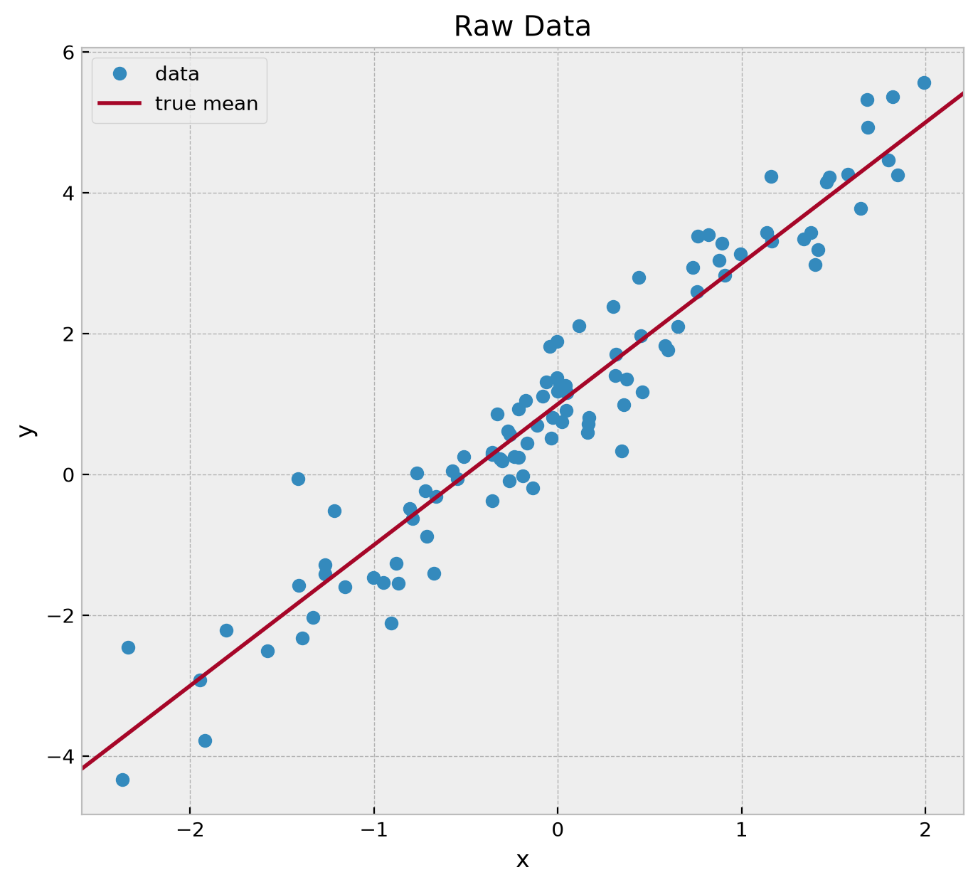
We generate some data from a simple linear regression model.
[4]:
def generate_data(rng_key, a, b, sigma, n):
    x = random.normal(rng_key, (n,))
    rng_key, rng_subkey = random.split(rng_key)
    epsilon = sigma * random.normal(rng_subkey, (n,))
    y = a + b * x + epsilon
    return x, y


# true parameters
a = 1.0
b = 2.0
sigma = 0.5
n = 100

# generate data
rng_key, rng_subkey = random.split(rng_key)
x, y = generate_data(rng_key, a, b, sigma, n)

# plot data
fig, ax = plt.subplots(figsize=(8, 7))
ax.plot(x, y, "o", c="C0", label="data")
ax.axline((0, a), slope=b, color="C1", label="true mean")
ax.legend(loc="upper left")
ax.set(xlabel="x", ylabel="y", title="Raw Data");
Model Specification
We define a simple linear regression model in NumPyro.
[5]:
def model(x, y=None):
    a = numpyro.sample("a", dist.Normal(loc=0.0, scale=2.0))
    b = numpyro.sample("b", dist.HalfNormal(scale=2.0))
    sigma = numpyro.sample("sigma", dist.Exponential(rate=1.0))
    mean = numpyro.deterministic("mu", a + b * x)
    with numpyro.plate("data", len(x)):
        numpyro.sample("likelihood", dist.Normal(loc=mean, scale=sigma), obs=y)


numpyro.render_model(
    model=model,
    model_args=(x, y),
    render_distributions=True,
    render_params=True,
)
[5]:

Extract Model Ingredients
We call initialize_model to compile the model into a potential_fn, an unconstrained initial position, and a single-position postprocess callable. All the bookkeeping (binding the model args/kwargs, computing inverse transforms) happens inside this single call; negating potential_fn gives the log joint density.
[6]:
rng_key, rng_subkey = random.split(rng_key)
model_info = initialize_model(rng_subkey, model, model_args=(x, y))
The returned model_info object exposes everything we need:
model_info.potential_fn(position) -> float: the potential energy. Negate it to get the log joint density to pass to any external sampler.model_info.param_info.z: adictof unconstrained initial values, ready to feed to the sampler’sinit.model_info.postprocess_fn(position) -> dict: converts a single unconstrained sample back to the constrained space and addsdeterministicsites.model_info.model_trace: the underlying execution trace for power users that want raw handles.
Let’s extract an initial position from parameters.
[7]:
# get initial position
initial_position = model_info.param_info.z
initial_position
[7]:
{'a': Array(1.43019189, dtype=float64),
 'b': Array(0.30644639, dtype=float64),
 'sigma': Array(-0.72184641, dtype=float64)}
Remark Observe that the initial position of sigma is negative. The reason is that the prior distribution for sigma is dist.Exponential(rate=1.0), which is a positive distribution. Hence, we need to transform it to an unconstrained space through a bijective transformation. The function postprocess_fn will transform this negative value to the positive space using the inverse transform.
We build the log-density function by negating model_info.potential_fn (the potential energy):
[8]:
def logdensity_fn(position):
    return -model_info.potential_fn(position)
Let’s verify we can evaluate the log-density function at the initial position.
[9]:
logdensity_fn(initial_position)
[9]:
Array(-229.21544977, dtype=float64)
Now, we are ready to run our first sampler.
Pathfinder Sampler
From Blackjax documentation:
Pathfinder locates normal approximations to the target density along a quasi-Newton optimization path, with local covariance estimated using the inverse Hessian estimates produced by the L-BFGS optimizer. PathfinderState stores for an interation fo the L-BFGS optimizer the resulting ELBO and all factors needed to sample from the approximated target density.
For more information about Pathfinder, please refer to the paper:
Lu Zhang, Bob Carpenter, Andrew Gelman, and Aki Vehtari. Pathfinder: parallel quasi-newton variational inference. Journal of Machine Learning Research, 23(306):1–49, 2022.
Remark: From Blackjax’s sampling book documentation:
L-BFGS algorithm struggles with float32s and log-likelihood functions; it’s suggested to use double precision numbers.
Run Sampler
We can now use blackjax.vi.pathfinder.approximate to run the variational inference algorithm.
[10]:
%%time

# run pathfinder
rng_key, rng_subkey = random.split(rng_key)
pathfinder_state, _ = blackjax.vi.pathfinder.approximate(
    rng_key=rng_subkey,
    logdensity_fn=logdensity_fn,
    initial_position=initial_position,
    num_samples=15_000,
    ftol=1e-4,
)

# sample from the posterior
rng_key, rng_subkey = random.split(rng_key)
posterior_samples_pathfinder, _ = blackjax.vi.pathfinder.sample(
    rng_key=rng_subkey,
    state=pathfinder_state,
    num_samples=5_000,
)

# convert to arviz
idata_pathfinder = az.from_dict(
    posterior={
        k: np.expand_dims(a=np.asarray(v), axis=0)
        for k, v in posterior_samples_pathfinder.items()
    },
)
CPU times: user 4.9 s, sys: 521 ms, total: 5.42 s
Wall time: 3.48 s
Visualize Results
We can visualize the results after sampling.
[11]:
az.summary(data=idata_pathfinder, round_to=3)
arviz - WARNING - Shape validation failed: input_shape: (1, 5000), minimum_shape: (chains=2, draws=4)
[11]:
| mean | sd | hdi_3% | hdi_97% | mcse_mean | mcse_sd | ess_bulk | ess_tail | r_hat | |
|---|---|---|---|---|---|---|---|---|---|
| a | 0.984 | 0.050 | 0.893 | 1.081 | 0.001 | 0.001 | 4672.592 | 4890.604 | NaN |
| b | 0.717 | 0.028 | 0.663 | 0.768 | 0.000 | 0.000 | 4928.670 | 4310.808 | NaN |
| sigma | -0.573 | 0.072 | -0.708 | -0.440 | 0.001 | 0.001 | 4632.030 | 4978.413 | NaN |
[12]:
axes = az.plot_trace(
    data=idata_pathfinder,
    compact=True,
    figsize=(10, 6),
    backend_kwargs={"layout": "constrained"},
)
plt.gcf().suptitle(
    t="Pathfinder Trace - Transformed Space", fontsize=18, fontweight="bold"
);
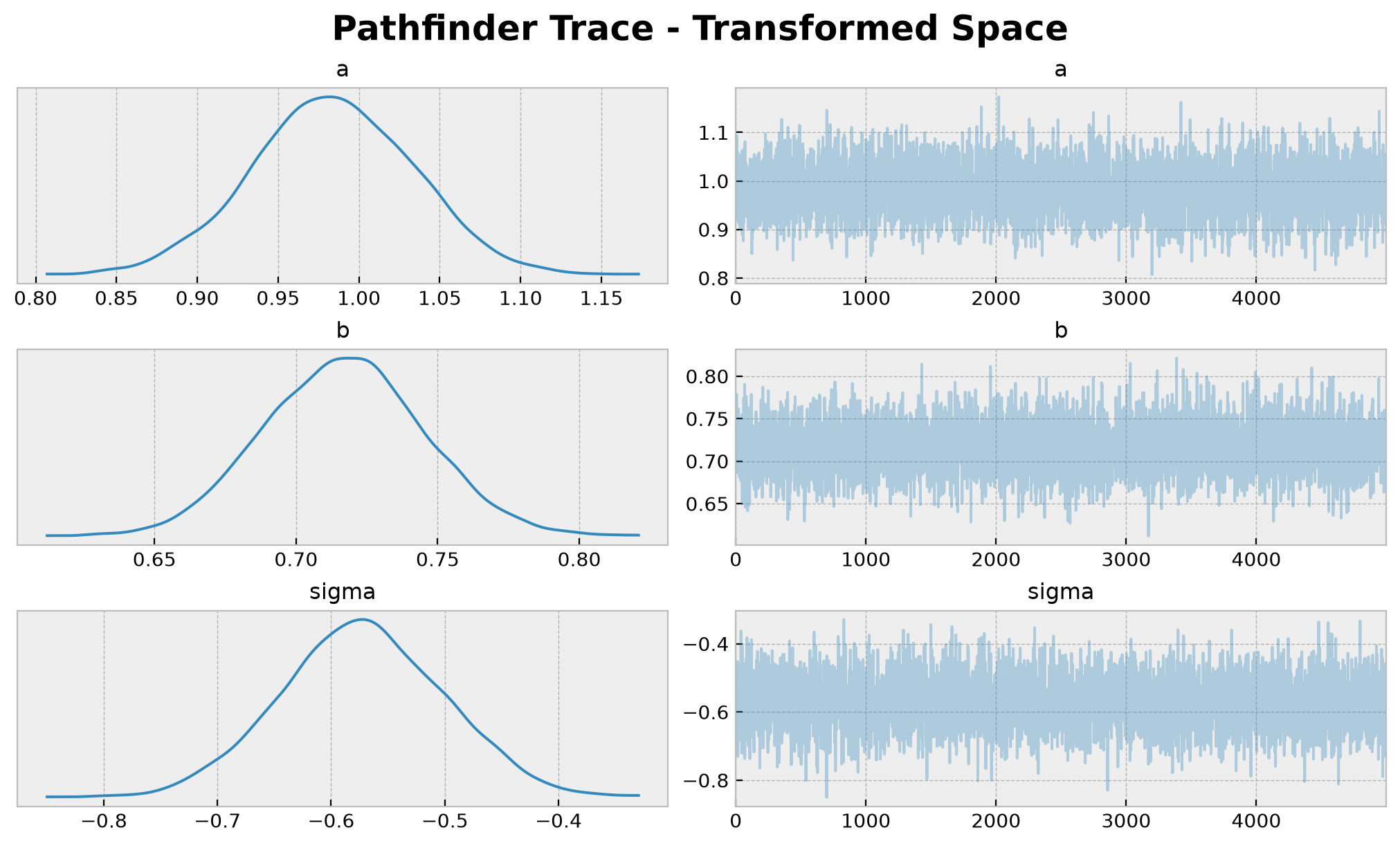
Note that the value for a is close to the true value of 1.0. However, the values for b and sigma do not match the true values of 2.0 and 0.5 respectively. Again, the reason is that we are working in the unconstrained space. We need to transform the samples to the original space to compare them with the true values.
Transform Samples
constrain_fn with batch_ndims=1 applies the inverse transforms (and adds deterministic sites) across the whole chain in one call; replacing the jax.vmap(postprocess_fn(...)) boilerplate.
[13]:
# convert unconstrained samples to constrained + deterministic sites in one call
posterior_samples_pathfinder_transformed = constrain_fn(
    model,
    (x, y),
    {},
    posterior_samples_pathfinder,
    return_deterministic=True,
    batch_ndims=1,
)

# posterior predictive samples
rng_key, rng_subkey = random.split(rng_key)
posterior_predictive_samples_pathfinder_transformed = Predictive(
    model=model, posterior_samples=posterior_samples_pathfinder_transformed
)(rng_subkey, x)
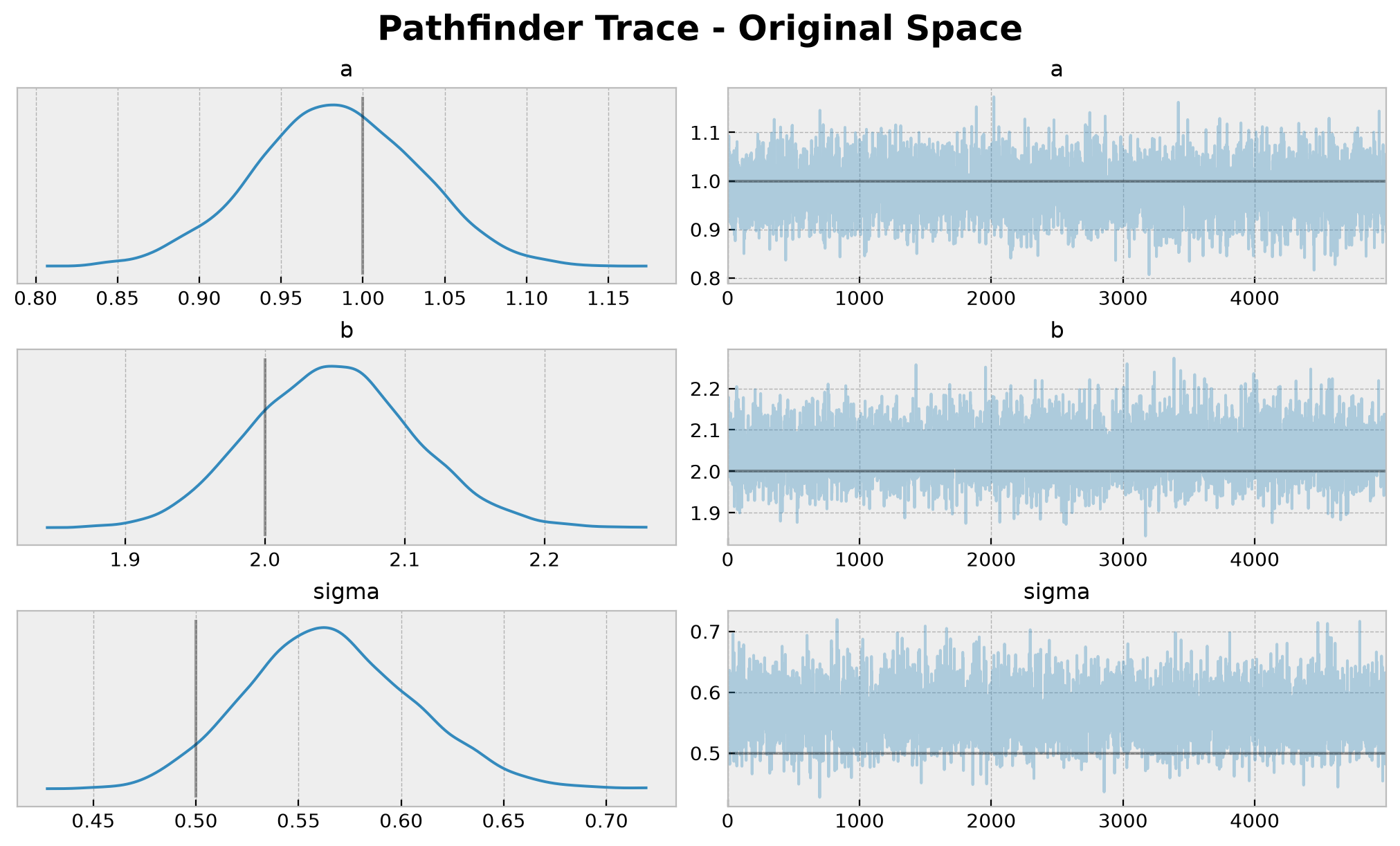
Let’s see the posterior distribution in the original space.
[14]:
idata_pathfinder_transformed = az.from_dict(
    posterior={
        k: np.expand_dims(a=np.asarray(v), axis=0)
        for k, v in posterior_samples_pathfinder_transformed.items()
    },
    posterior_predictive={
        k: np.expand_dims(a=np.asarray(v), axis=0)
        for k, v in posterior_predictive_samples_pathfinder_transformed.items()
    },
)

axes = az.plot_trace(
    data=idata_pathfinder_transformed,
    var_names=["~mu"],
    compact=True,
    figsize=(10, 6),
    lines=[
        ("a", {}, a),
        ("b", {}, b),
        ("sigma", {}, sigma),
    ],
    backend_kwargs={"layout": "constrained"},
)
plt.gcf().suptitle(
    t="Pathfinder Trace - Original Space", fontsize=18, fontweight="bold"
);
Finally, we can visualize the posterior predictive distribution.
[15]:
fig, ax = plt.subplots(figsize=(7, 6))
ax.plot(x, y, "o", c="C0", label="data")
ax.axline((0, a), slope=b, color="C1", label="true mean")
az.plot_hdi(
    x=x,
    y=idata_pathfinder_transformed["posterior_predictive"]["mu"],
    color="C2",
    fill_kwargs={"alpha": 0.7, "label": "mu posterior ($94\\%$ HDI)"},
    ax=ax,
)
az.plot_hdi(
    x=x,
    y=idata_pathfinder_transformed["posterior_predictive"]["likelihood"],
    color="C2",
    fill_kwargs={"alpha": 0.2, "label": "posterior predictive ($94\\%$ HDI)"},
    ax=ax,
)
ax.legend(loc="upper left")
ax.set(xlabel="x", ylabel="y", title="Pathfinder Posterior Predictive");
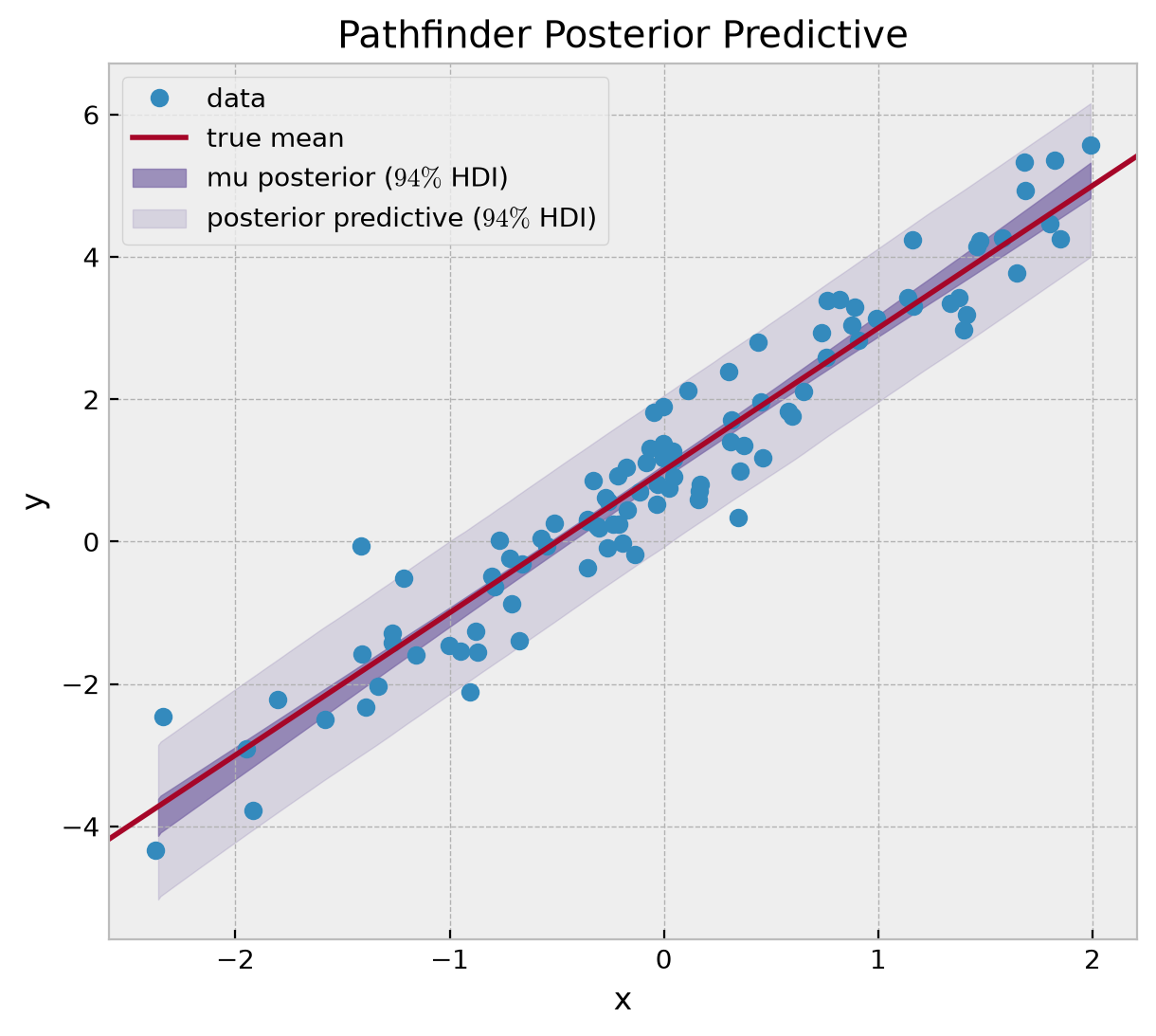
The results look good!
MCLMC Sampler via a custom MCMCKernel
Microcanonical Langevin Monte Carlo (MCLMC) is a full MCMC sampler implemented in Blackjax. Unlike Pathfinder, which is a one-shot variational method, MCLMC produces a long Markov chain that we want to drive through NumPyro’s MCMC class to get the progress bar, multi-chain support, and seamless Predictive integration.
Rather than introducing a bespoke adapter class, we simply subclass numpyro.infer.mcmc.MCMCKernel directly. This keeps full control over the sampler’s state and step, and the model-side plumbing (log-density, initial position, and postprocess back to the constrained space with deterministic sites) comes from initialize_model (negating potential_fn for the log-density).
Define the MCMCKernel subclass
A NumPyro MCMCKernel needs three things: an init method that builds the initial state, a sample method that advances the chain by one step, and a sample_field telling MCMC which attribute of the state holds the sample.
Inside init we call initialize_model, build logdensity_fn by negating potential_fn, read the unconstrained initial position from param_info.z, and expose the single-position postprocess_fn. The MCLMC adaptation that tunes L and step_size also runs here. We expose the postprocess via postprocess_fn so MCMC maps the samples back to the constrained space (including the deterministic mu site).
This kernel holds its step and postprocess functions on the instance (set in init), so it works for single-chain runs and for chain_method="sequential" or "parallel", where each chain runs its own init. It does not support chain_method="vectorized", which would vmap init across chains.
[ ]:
MCLMCState = namedtuple("MCLMCState", ["position", "inner", "rng_key"])


class BlackjaxMCLMCKernel(MCMCKernel):
    """Drive Blackjax MCLMC through NumPyro's `MCMC` by subclassing `MCMCKernel`.

    The model-side plumbing (log-density, init position, postprocess back to the
    constrained space with deterministic sites) comes from `initialize_model`;
    the MCLMC tuning lives in `init`.
    """

    sample_field = "position"

    def __init__(self, model, num_tuning_steps=2_000, init_strategy=init_to_uniform):
        self._model = model
        self._num_tuning_steps = num_tuning_steps
        self._init_strategy = init_strategy
        self._step_fn = None
        self._postprocess_fn = None

    def postprocess_fn(self, model_args, model_kwargs):
        return self._postprocess_fn

    def init(self, rng_key, num_warmup, init_params, model_args, model_kwargs):
        key_model, key_init, key_tune = random.split(rng_key, 3)
        model_info = initialize_model(
            key_model,
            self._model,
            init_strategy=self._init_strategy,
            model_args=model_args,
            model_kwargs=model_kwargs,
        )

        def logdensity_fn(position):
            return -model_info.potential_fn(position)

        self._postprocess_fn = model_info.postprocess_fn
        init_position = model_info.param_info.z if init_params is None else init_params

        init_state = blackjax.mcmc.mclmc.init(
            position=init_position, logdensity_fn=logdensity_fn, rng_key=key_init
        )

        def kernel_factory(inverse_mass_matrix):
            return blackjax.mcmc.mclmc.build_kernel(
                logdensity_fn=logdensity_fn,
                inverse_mass_matrix=inverse_mass_matrix,
                integrator=isokinetic_mclachlan,
            )

        tuned_state, params, _ = blackjax.mclmc_find_L_and_step_size(
            mclmc_kernel=kernel_factory,
            num_steps=self._num_tuning_steps,
            state=init_state,
            rng_key=key_tune,
        )
        final_kernel = kernel_factory(params.inverse_mass_matrix)

        def step_fn(rng_key, state):
            return final_kernel(rng_key, state, params.L, params.step_size)

        self._step_fn = step_fn
        return MCLMCState(tuned_state.position, tuned_state, rng_key)

    def sample(self, state, model_args, model_kwargs):
        rng_key, step_key = random.split(state.rng_key)
        new_inner, _ = self._step_fn(step_key, state.inner)
        return MCLMCState(new_inner.position, new_inner, rng_key)
Run the sampler via MCMC
Pass num_warmup=0 to MCMC, the warmup budget is baked into the build_kernel closure above. The rest is identical to running any other NumPyro sampler.
[17]:
%%time

rng_key, rng_subkey = random.split(rng_key)
mcmc_mclmc = MCMC(
    BlackjaxMCLMCKernel(model, num_tuning_steps=2_000),
    num_warmup=0,
    num_samples=5_000,
    progress_bar=False,
)
mcmc_mclmc.run(rng_subkey, x, y)
posterior_samples_mclmc = mcmc_mclmc.get_samples()
CPU times: user 4.91 s, sys: 251 ms, total: 5.16 s
Wall time: 2.39 s
get_samples() returns constrained samples with deterministic sites already included, ready for arviz and Predictive without any extra post-processing.
[18]:
rng_key, rng_subkey = random.split(rng_key)
posterior_predictive_mclmc = Predictive(
    model=model, posterior_samples=posterior_samples_mclmc
)(rng_subkey, x)

idata_mclmc = az.from_dict(
    posterior={
        k: np.expand_dims(np.asarray(v), axis=0)
        for k, v in posterior_samples_mclmc.items()
    },
    posterior_predictive={
        k: np.expand_dims(np.asarray(v), axis=0)
        for k, v in posterior_predictive_mclmc.items()
    },
)

az.summary(data=idata_mclmc, var_names=["a", "b", "sigma"], round_to=3)
arviz - WARNING - Shape validation failed: input_shape: (1, 5000), minimum_shape: (chains=2, draws=4)
[18]:
| mean | sd | hdi_3% | hdi_97% | mcse_mean | mcse_sd | ess_bulk | ess_tail | r_hat | |
|---|---|---|---|---|---|---|---|---|---|
| a | 0.990 | 0.056 | 0.881 | 1.092 | 0.001 | 0.001 | 1783.709 | 2265.997 | NaN |
| b | 2.047 | 0.057 | 1.941 | 2.152 | 0.002 | 0.001 | 1297.571 | 1898.786 | NaN |
| sigma | 0.571 | 0.041 | 0.497 | 0.646 | 0.001 | 0.001 | 2033.627 | 2780.921 | NaN |
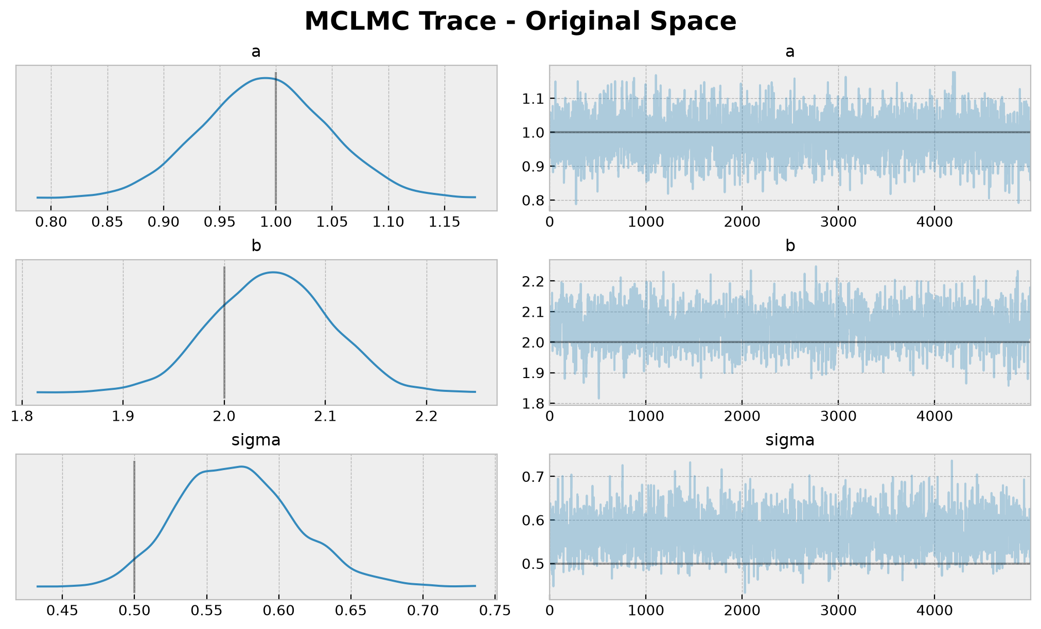
[19]:
axes = az.plot_trace(
    data=idata_mclmc,
    var_names=["~mu"],
    compact=True,
    figsize=(10, 6),
    lines=[
        ("a", {}, a),
        ("b", {}, b),
        ("sigma", {}, sigma),
    ],
    backend_kwargs={"layout": "constrained"},
)
plt.gcf().suptitle(t="MCLMC Trace - Original Space", fontsize=18, fontweight="bold");
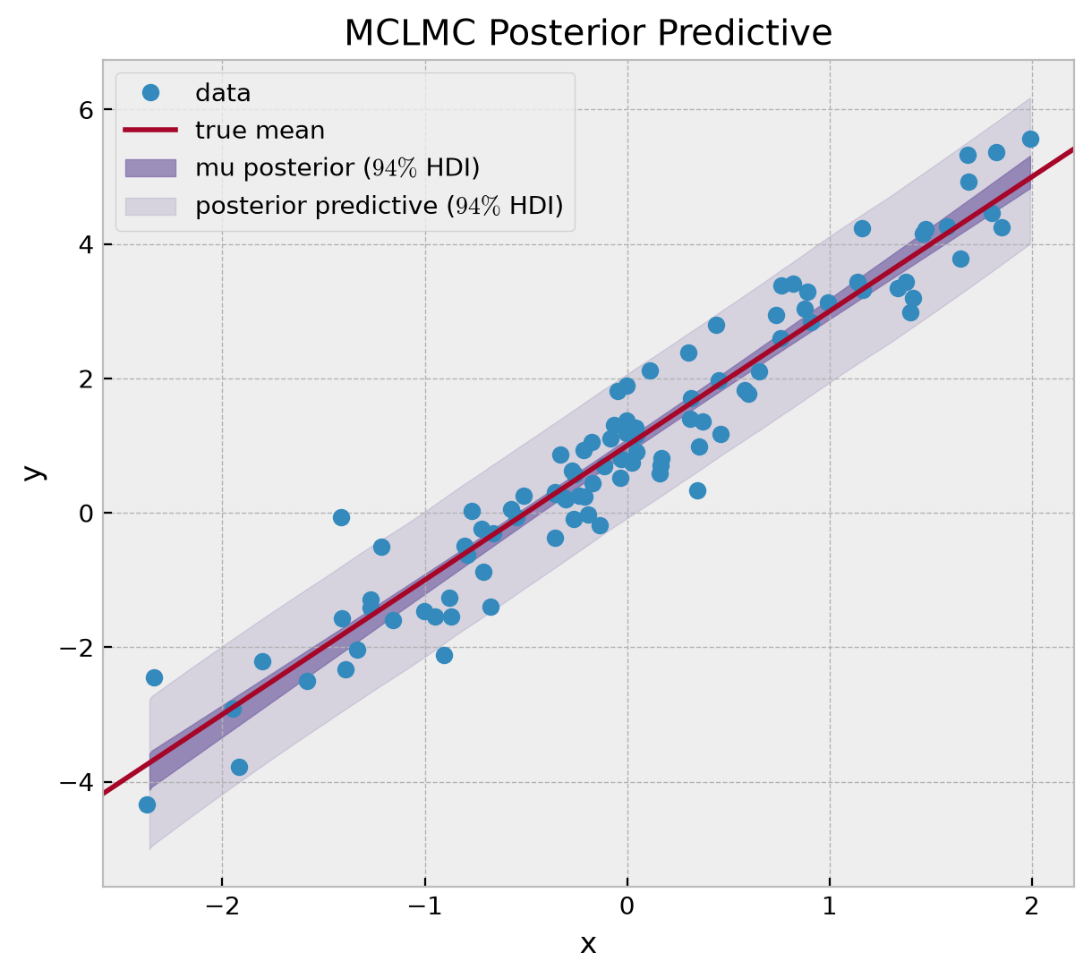
[20]:
fig, ax = plt.subplots(figsize=(7, 6))
ax.plot(x, y, "o", c="C0", label="data")
ax.axline((0, a), slope=b, color="C1", label="true mean")
az.plot_hdi(
    x=x,
    y=idata_mclmc["posterior_predictive"]["mu"],
    color="C2",
    fill_kwargs={"alpha": 0.7, "label": "mu posterior ($94\\%$ HDI)"},
    ax=ax,
)
az.plot_hdi(
    x=x,
    y=idata_mclmc["posterior_predictive"]["likelihood"],
    color="C2",
    fill_kwargs={"alpha": 0.2, "label": "posterior predictive ($94\\%$ HDI)"},
    ax=ax,
)
ax.legend(loc="upper left")
ax.set(xlabel="x", ylabel="y", title="MCLMC Posterior Predictive");
FlowMC Normalizing Flow Sampler
We can run the FlowMC sampler in a similar way as above. We just need to adapt the log-density function to the FlowMC format.
Define Log-Density Function
[21]:
def logdensity_fn_flowmc(position, data):
    """FlowMC passes positions as an (n_chains, n_dim) array. Reshape into
    the pytree NumPyro expects, then call the precomputed logdensity_fn."""
    dict_position = dict(zip(initial_position.keys(), position[..., None]))
    return logdensity_fn(dict_position)
Let’s verify that the log-density function is working.
[22]:
n_dim = 3  # number of parameters
n_chains = 20  # number of chains
[23]:
data = {"x": x, "y": y}
rng_key, subkey = random.split(rng_key)
initial_position_array = jax.random.normal(subkey, shape=(n_chains, n_dim))
[24]:
logdensity_fn_flowmc(initial_position_array, data)
[24]:
Array(-686.62149936, dtype=float64)
Define FlowMC Sampler
FlowMC 0.5 reorganised its API around the ResourceStrategyBundle pattern: one bundle constructor wires up the local MALA proposal, the RQ-spline normalising flow, and the sampling strategies. The user-facing Sampler only needs the bundle. See the flowMC documentation for the full reference.
[ ]:
%%time

rng_key, key_bundle, key_sampler = random.split(rng_key, 3)

bundle = RQSpline_MALA_Bundle(
    rng_key=key_bundle,
    n_chains=n_chains,
    n_dims=n_dim,
    logpdf=logdensity_fn_flowmc,
    n_local_steps=150,
    n_global_steps=100,
    n_training_loops=7,
    n_production_loops=7,
    n_epochs=30,
    learning_rate=0.001,
    batch_size=10_000,
    rq_spline_hidden_units=[32, 32],
    rq_spline_n_layers=4,
    rq_spline_n_bins=8,
    mala_step_size=0.1,
)

nf_sampler = Sampler(
    n_dim=n_dim,
    n_chains=n_chains,
    rng_key=key_sampler,
    resource_strategy_bundles=bundle,
)

nf_sampler.sample(initial_position_array, data)

# Production buffer shape: (n_chains, n_steps, n_dim). Flatten to one big batch
# so the downstream cells (which already expect a 2-D (N, n_dim) array) keep
# working unchanged.
production = nf_sampler.resources["positions_production"].data
nf_samples = production.reshape(-1, n_dim)
Visualize Results
We collect the posterior samples and visualize the results.
[ ]:
posterior_samples_flowmc = dict(zip(initial_position.keys(), nf_samples.T))

flowmc_idata = az.from_dict(posterior=posterior_samples_flowmc)
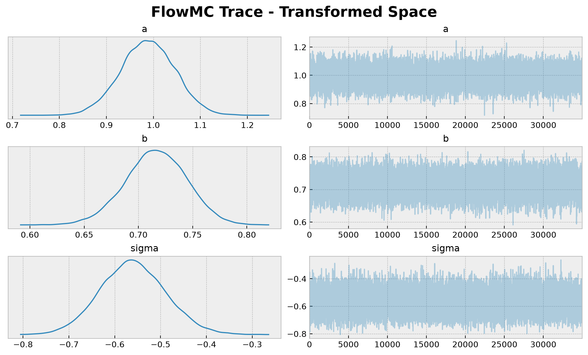
[28]:
axes = az.plot_trace(
    data=flowmc_idata,
    compact=True,
    figsize=(10, 6),
    backend_kwargs={"layout": "constrained"},
)
plt.gcf().suptitle(
    t="FlowMC Trace - Transformed Space", fontsize=18, fontweight="bold"
);
Transform Samples
Same one-call transform as Pathfinder.
[ ]:
# posterior samples: use constrain_fn instead of jax.vmap(postprocess_fn(...))
posterior_samples_flowmc_transformed = constrain_fn(
    model,
    (x, y),
    {},
    posterior_samples_flowmc,
    return_deterministic=True,
    batch_ndims=1,
)

# posterior predictive samples
rng_key, rng_subkey = random.split(rng_key)
posterior_predictive_samples_flowmc_transformed = Predictive(
    model=model, posterior_samples=posterior_samples_flowmc_transformed
)(rng_subkey, x)
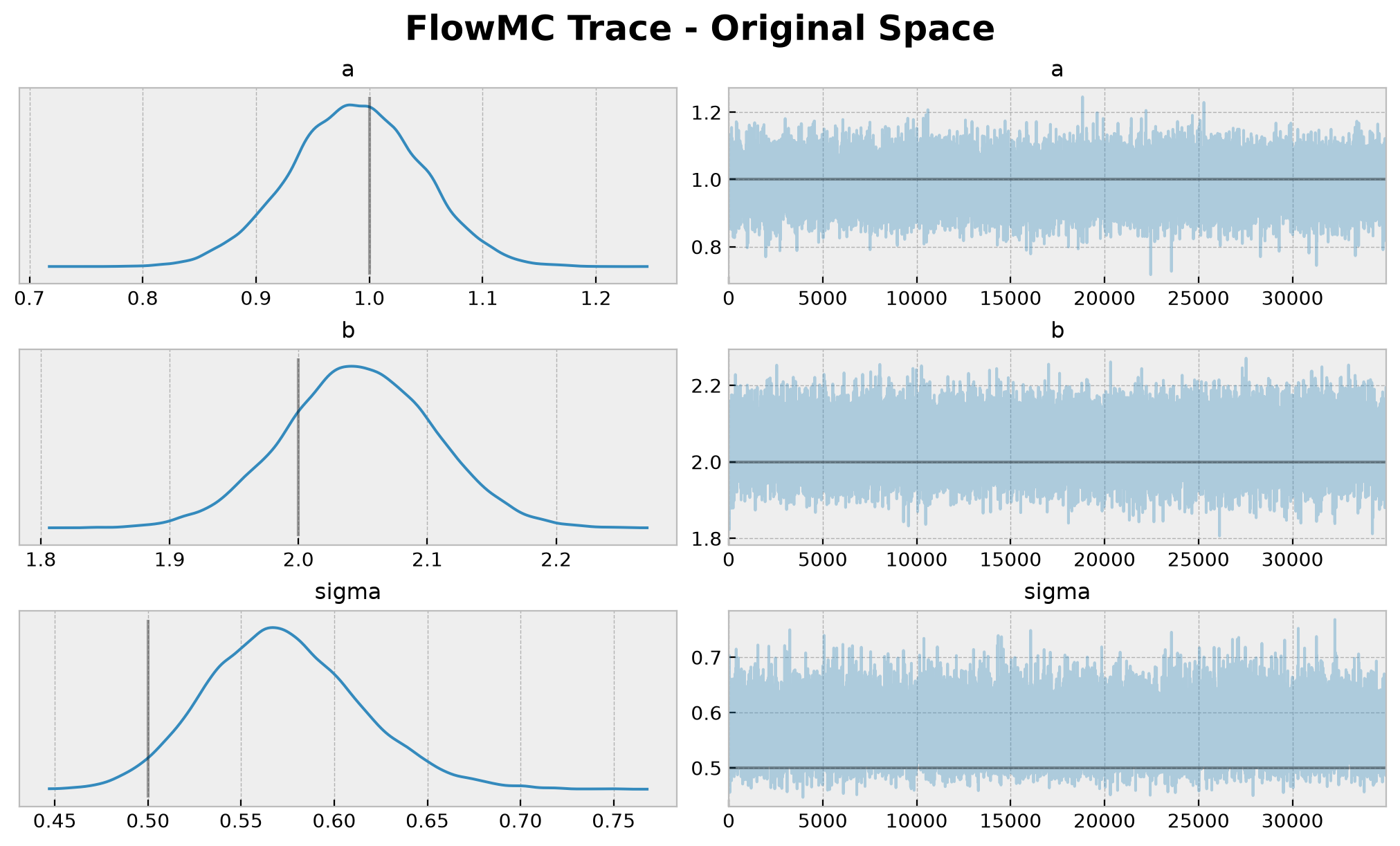
[30]:
idata_flowmc_transformed = az.from_dict(
    posterior={
        k: np.expand_dims(a=np.asarray(v), axis=0)
        for k, v in posterior_samples_flowmc_transformed.items()
    },
    posterior_predictive={
        k: np.expand_dims(a=np.asarray(v), axis=0)
        for k, v in posterior_predictive_samples_flowmc_transformed.items()
    },
)

axes = az.plot_trace(
    data=idata_flowmc_transformed,
    var_names=["~mu"],
    compact=True,
    figsize=(10, 6),
    lines=[
        ("a", {}, a),
        ("b", {}, b),
        ("sigma", {}, sigma),
    ],
    backend_kwargs={"layout": "constrained"},
)
plt.gcf().suptitle(t="FlowMC Trace - Original Space", fontsize=18, fontweight="bold");
[31]:
fig, ax = plt.subplots(figsize=(7, 6))
ax.plot(x, y, "o", c="C0", label="data")
ax.axline((0, a), slope=b, color="C1", label="true mean")
az.plot_hdi(
    x=x,
    y=idata_flowmc_transformed["posterior_predictive"]["mu"],
    color="C2",
    fill_kwargs={"alpha": 0.7, "label": "mu posterior ($94\\%$ HDI)"},
    ax=ax,
)
az.plot_hdi(
    x=x,
    y=idata_flowmc_transformed["posterior_predictive"]["likelihood"],
    color="C2",
    fill_kwargs={"alpha": 0.2, "label": "posterior predictive ($94\\%$ HDI)"},
    ax=ax,
)
ax.legend(loc="upper left")
ax.set(xlabel="x", ylabel="y", title="FlowMC Posterior Predictive");

Model Comparison
Finally, we compare the results of the two samplers.
[32]:
az.plot_forest(
    data=[idata_pathfinder_transformed, idata_mclmc, idata_flowmc_transformed],
    model_names=["Pathfinder", "MCLMC", "FlowMC"],
    var_names=["a", "b", "sigma"],
    combined=True,
    figsize=(8, 5),
    backend_kwargs={"layout": "constrained"},
);
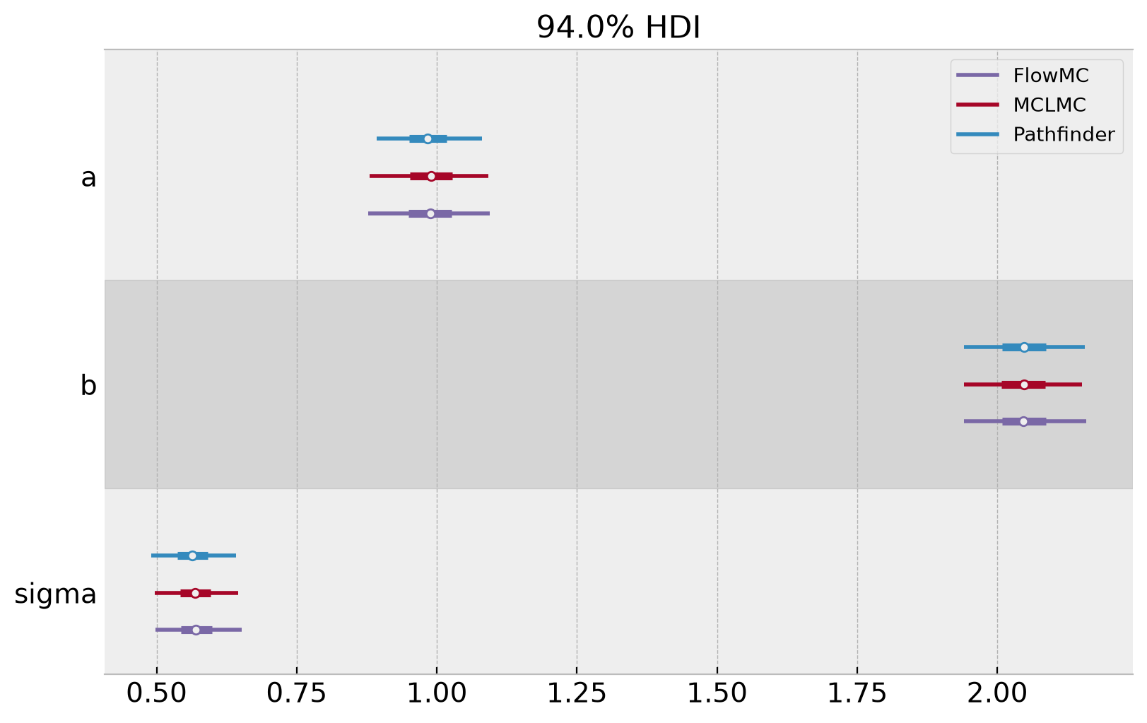
All three samplers recover the synthetic-data parameters. MCLMC, via a small MCMCKernel subclass, gets the benefit of NumPyro’s full MCMC pipeline with just a handful of lines of glue.
Remark: We would like to mention a relevant project that helps fitting NumPyro models with other inference algorithms:
bayeux lets you write a probabilistic model in JAX and immediately have access to state-of-the-art inference methods. The API aims to be simple, self descriptive, and helpful. Simply provide a log density function (which doesn’t even have to be normalized), along with a single point (specified as a pytree) where that log density is finite. Then let bayeux do the rest!
Check it out!