Example: Predator-Prey Model

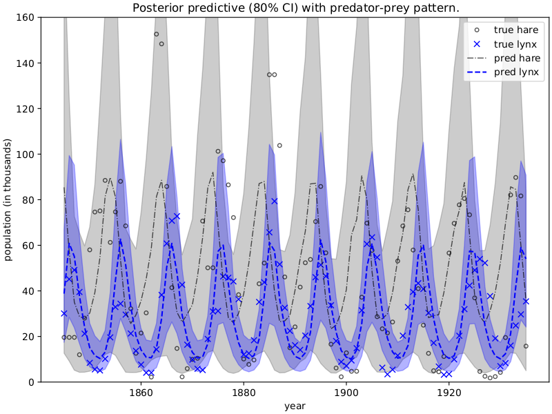
This example replicates the great case study [1], which leverages the Lotka-Volterra equation [2] to describe the dynamics of Canada lynx (predator) and snowshoe hare (prey) populations. We will use the dataset obtained from [3] and run MCMC to get inferences about parameters of the differential equation governing the dynamics.

References:

1. Bob Carpenter (2018), “Predator-Prey Population Dynamics: the Lotka-Volterra model in Stan”.
2. https://en.wikipedia.org/wiki/Lotka-Volterra_equations
3. http://people.whitman.edu/~hundledr/courses/M250F03/M250.html

import argparse
import os

import matplotlib
import matplotlib.pyplot as plt

from jax.experimental.ode import odeint
import jax.numpy as jnp
from jax.random import PRNGKey

import numpyro
import numpyro.distributions as dist
from numpyro.examples.datasets import LYNXHARE, load_dataset
from numpyro.infer import MCMC, NUTS, Predictive

matplotlib.use("Agg")  # noqa: E402


def dz_dt(z, t, theta):
    """
    Lotka–Volterra equations. Real positive parameters `alpha`, `beta`, `gamma`, `delta`
    describes the interaction of two species.
    """
    u = z[0]
    v = z[1]
    alpha, beta, gamma, delta = (
        theta[..., 0],
        theta[..., 1],
        theta[..., 2],
        theta[..., 3],
    )
    du_dt = (alpha - beta * v) * u
    dv_dt = (-gamma + delta * u) * v
    return jnp.stack([du_dt, dv_dt])


def model(N, y=None):
    """
    :param int N: number of measurement times
    :param numpy.ndarray y: measured populations with shape (N, 2)
    """
    # initial population
    z_init = numpyro.sample("z_init", dist.LogNormal(jnp.log(10), 1).expand([2]))
    # measurement times
    ts = jnp.arange(float(N))
    # parameters alpha, beta, gamma, delta of dz_dt
    theta = numpyro.sample(
        "theta",
        dist.TruncatedNormal(
            low=0.0,
            loc=jnp.array([1.0, 0.05, 1.0, 0.05]),
            scale=jnp.array([0.5, 0.05, 0.5, 0.05]),
        ),
    )
    # integrate dz/dt, the result will have shape N x 2
    z = odeint(dz_dt, z_init, ts, theta, rtol=1e-6, atol=1e-5, mxstep=1000)
    # measurement errors
    sigma = numpyro.sample("sigma", dist.LogNormal(-1, 1).expand([2]))
    # measured populations
    numpyro.sample("y", dist.LogNormal(jnp.log(z), sigma), obs=y)


def main(args):
    _, fetch = load_dataset(LYNXHARE, shuffle=False)
    year, data = fetch()  # data is in hare -> lynx order

    # use dense_mass for better mixing rate
    mcmc = MCMC(
        NUTS(model, dense_mass=True),
        num_warmup=args.num_warmup,
        num_samples=args.num_samples,
        num_chains=args.num_chains,
        progress_bar=False if "NUMPYRO_SPHINXBUILD" in os.environ else True,
    )
    mcmc.run(PRNGKey(1), N=data.shape[0], y=data)
    mcmc.print_summary()

    # predict populations
    pop_pred = Predictive(model, mcmc.get_samples())(PRNGKey(2), data.shape[0])["y"]
    mu = jnp.mean(pop_pred, 0)
    pi = jnp.percentile(pop_pred, jnp.array([10, 90]), 0)
    plt.figure(figsize=(8, 6), constrained_layout=True)
    plt.plot(year, data[:, 0], "ko", mfc="none", ms=4, label="true hare", alpha=0.67)
    plt.plot(year, data[:, 1], "bx", label="true lynx")
    plt.plot(year, mu[:, 0], "k-.", label="pred hare", lw=1, alpha=0.67)
    plt.plot(year, mu[:, 1], "b--", label="pred lynx")
    plt.fill_between(year, pi[0, :, 0], pi[1, :, 0], color="k", alpha=0.2)
    plt.fill_between(year, pi[0, :, 1], pi[1, :, 1], color="b", alpha=0.3)
    plt.gca().set(ylim=(0, 160), xlabel="year", ylabel="population (in thousands)")
    plt.title("Posterior predictive (80% CI) with predator-prey pattern.")
    plt.legend()

    plt.savefig("ode_plot.pdf")


if __name__ == "__main__":
    assert numpyro.__version__.startswith("0.11.0")
    parser = argparse.ArgumentParser(description="Predator-Prey Model")
    parser.add_argument("-n", "--num-samples", nargs="?", default=1000, type=int)
    parser.add_argument("--num-warmup", nargs="?", default=1000, type=int)
    parser.add_argument("--num-chains", nargs="?", default=1, type=int)
    parser.add_argument("--device", default="cpu", type=str, help='use "cpu" or "gpu".')
    args = parser.parse_args()

    numpyro.set_platform(args.device)
    numpyro.set_host_device_count(args.num_chains)

    main(args)