Truncated and folded distributions
This tutorial will cover how to work with truncated and folded distributions in NumPyro. It is assumed that you’re already familiar with the basics of NumPyro. To get the most out of this tutorial you’ll need some background in probability.
Table of contents
Setup
To run this notebook, we are going to need the following imports
[ ]:
!pip install -q git+https://github.com/pyro-ppl/numpyro.git
[2]:
import matplotlib.pyplot as plt
import numpy as np
from scipy.stats import poisson as sp_poisson

import jax
from jax import lax, random
import jax.numpy as jnp
from jax.scipy.special import ndtri
from jax.scipy.stats import norm, poisson

import numpyro
import numpyro.distributions as dist
from numpyro.distributions import (
    Distribution,
    FoldedDistribution,
    SoftLaplace,
    StudentT,
    TruncatedDistribution,
    TruncatedNormal,
    constraints,
)
from numpyro.distributions.util import promote_shapes
from numpyro.infer import MCMC, NUTS, DiscreteHMCGibbs, Predictive

numpyro.enable_x64()
RNG = random.key(0)
PRIOR_RNG, MCMC_RNG, PRED_RNG = random.split(RNG, 3)
MCMC_KWARGS = dict(
    num_warmup=2000,
    num_samples=2000,
    num_chains=4,
    chain_method="sequential",
)
1. What are truncated distributions?
The support of a probability distribution is the set of values in the domain with non-zero probability. For example, the support of the normal distribution is the whole real line (even if the density gets very small as we move away from the mean, technically speaking, it is never quite zero). The support of the uniform distribution, as coded in jax.random.uniform with the default arguments, is the interval \(\left[0, 1)\right.\), because any value outside of that interval has
zero probability. The support of the Poisson distribution is the set of non-negative integers, etc.
Truncating a distribution makes its support smaller so that any value outside our desired domain has zero probability. In practice, this can be useful for modelling situations in which certain biases are introduced during data collection. For example, some physical detectors only get triggered when the signal is above some minimum threshold, or sometimes the detectors fail if the signal exceeds a certain value. As a result, the observed values are constrained to be within a limited range of values, even though the true signal does not have the same constraints. See, for example, section 3.1 of Information Theory and Learning Algorithms by David Mackay. Naively, if \(S\) is the support of the original density \(p_Y(y)\), then by truncating to a new support \(T\subset S\) we are effectively defining a new random variable \(Z\) for which the density is
The reason for writing a \(\propto\) (proportional to) sign instead of a strict equation is that, defined in the above way, the resulting function does not integrate to \(1\) and so it cannot be strictly considered a probability density. To make it into a probability density we need to re-distribute the truncated mass among the part of the distribution that remains. To do this, we simply re-weight every point by the same constant:
where \(M = \int_T p_Y(y)\mathrm{d}y\).
In practice, the truncation is often one-sided. This means that if, for example, the support before truncation is the interval \((a, b)\), then the support after truncation is of the form \((a, c)\) or \((c, b)\), with \(a < c < b\). The figure below illustrates a left-sided truncation at zero of a normal distribution \(N(1, 1)\).

The original distribution (left side) is truncated at the vertical dotted line. The truncated mass (orange region) is redistributed in the new support (right side image) so that the total area under the curve remains equal to 1 even after truncation. This method of re-weighting ensures that the density ratio between any two points, \(p(a)/p(b)\) remains the same before and after the reweighting is done (as long as the points are inside the new support, of course).
Note: Truncated data is different from censored data. Censoring also hides values that are outside some desired support but, contrary to truncated data, we know when a value has been censored. The typical example is the household scale which does not report values above 300 pounds. Censored data will not be covered in this tutorial.
2. What is a folded distribution?
Folding is achieved by taking the absolute value of a random variable, \(Z = \lvert Y \rvert\). This obviously modifies the support of the original distribution since negative values now have zero probability:
The figure below illustrates a folded normal distribution \(N(1, 1)\).

As you can see, the resulting distribution is different from the truncated case. In particular, the density ratio between points, \(p(a)/p(b)\), is in general not the same after folding. For some examples in which folding is relevant see references 3 and 4
If the original distribution is symmetric around zero, then folding and truncating at zero have the same effect.
3. Sampling from truncated and folded distributions
Truncated distributions
Usually, we already have a sampler for the pre-truncated distribution (e.g. np.random.normal). So, a seemingly simple way of generating samples from the truncated distribution would be to sample from the original distribution, and then discard the samples that are outside the desired support. For example, if we wanted samples from a normal distribution truncated to the support \((-\infty, 1)\), we’d simply do:
upper = 1
samples = np.random.normal(size=1000)
truncated_samples = samples[samples < upper]
This is called rejection sampling but it is not very efficient. If the region we truncated had a sufficiently high probability mass, then we’d be discarding a lot of samples and it might be a while before we accumulate sufficient samples for the truncated distribution. For example, the above snippet would only result in approximately 840 truncated samples even though we initially drew 1000. This can easily get a lot worse for other combinations of parameters. A more efficient approach is to use a method known as inverse transform sampling. In this method, we first sample from a uniform distribution in (0, 1) and then transform those samples with the inverse cumulative distribution of our truncated distribution. This method ensures that no samples are wasted in the process, though it does have the slight complication that we need to calculate the inverse CDF (ICDF) of our truncated distribution. This might sound too complicated at first but, with a bit of algebra, we can often calculate the truncated ICDF in terms of the untruncated ICDF. The untruncated ICDF for many distributions is already available.
Folded distributions
This case is a lot simpler. Since we already have a sampler for the pre-folded distribution, all we need to do is to take the absolute value of those samples:
samples = np.random.normal(size=1000)
folded_samples = np.abs(samples)
4. Ready to use truncated and folded distributions
The later sections in this tutorial will show you how to construct your own truncated and folded distributions, but you don’t have to reinvent the wheel. NumPyro has a bunch of truncated distributions already implemented.
Suppose, for example, that you want a normal distribution truncated on the right. For that purpose, we use the TruncatedNormal distribution. The parameters of this distribution are loc and scale, corresponding to the loc and scale of the untruncated normal, and low and/or high corresponding to the truncation points. Importantly, the low and high are keyword only arguments, only loc
and scale are valid as positional arguments. This is how you can use this class in a model:
[3]:
def truncated_normal_model(num_observations, high, x=None):
    loc = numpyro.sample("loc", dist.Normal())
    scale = numpyro.sample("scale", dist.LogNormal())
    with numpyro.plate("observations", num_observations):
        numpyro.sample("x", TruncatedNormal(loc, scale, high=high), obs=x)
Let’s now check that we can use this model in a typical MCMC workflow.
Prior simulation
[4]:
high = 1.2
num_observations = 250
num_prior_samples = 100

prior = Predictive(truncated_normal_model, num_samples=num_prior_samples)
prior_samples = prior(PRIOR_RNG, num_observations, high)
Inference
To test our model, we run mcmc against some synthetic data. The synthetic data can be any arbitrary sample from the prior simulation.
[5]:
# -- select an arbitrary prior sample as true data
true_idx = 0
true_loc = prior_samples["loc"][true_idx]
true_scale = prior_samples["scale"][true_idx]
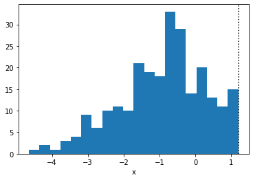
true_x = prior_samples["x"][true_idx]
[6]:
plt.hist(true_x.copy(), bins=20)
plt.axvline(high, linestyle=":", color="k")
plt.xlabel("x")
plt.show()
[7]:
# --- Run MCMC and check estimates and diagnostics
mcmc = MCMC(NUTS(truncated_normal_model), **MCMC_KWARGS)
mcmc.run(MCMC_RNG, num_observations, high, true_x)
mcmc.print_summary()

# --- Compare to ground truth
print(f"True loc  : {true_loc:3.2}")
print(f"True scale: {true_scale:3.2}")
sample: 100%|█████████████████████████████████████████████████████████████████████████████████████████████████████████████████████████| 4000/4000 [00:02<00:00, 1909.24it/s, 1 steps of size 5.65e-01. acc. prob=0.93]
sample: 100%|████████████████████████████████████████████████████████████████████████████████████████████████████████████████████████| 4000/4000 [00:00<00:00, 10214.14it/s, 3 steps of size 5.16e-01. acc. prob=0.95]
sample: 100%|████████████████████████████████████████████████████████████████████████████████████████████████████████████████████████| 4000/4000 [00:00<00:00, 15102.95it/s, 1 steps of size 6.42e-01. acc. prob=0.90]
sample: 100%|████████████████████████████████████████████████████████████████████████████████████████████████████████████████████████| 4000/4000 [00:00<00:00, 16522.03it/s, 3 steps of size 6.39e-01. acc. prob=0.90]
                mean       std    median      5.0%     95.0%     n_eff     r_hat
       loc     -0.58      0.15     -0.59     -0.82     -0.35   2883.69      1.00
     scale      1.49      0.11      1.48      1.32      1.66   3037.78      1.00

Number of divergences: 0
True loc  : -0.56
True scale: 1.4
Removing the truncation
Once we have inferred the parameters of our model, a common task is to understand what the data would look like without the truncation. In this example, this is easily done by simply “pushing” the value of high to infinity.
[8]:
pred = Predictive(truncated_normal_model, posterior_samples=mcmc.get_samples())
pred_samples = pred(PRED_RNG, num_observations, high=float("inf"))
Let’s finally plot these samples and compare them to the original, observed data.
[9]:
# thin the samples to not saturate matplotlib
samples_thinned = pred_samples["x"].ravel()[::1000]
[10]:
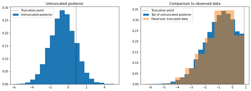
f, axes = plt.subplots(1, 2, figsize=(15, 5), sharex=True)

axes[0].hist(
    samples_thinned.copy(), label="Untruncated posterior", bins=20, density=True
)
axes[0].set_title("Untruncated posterior")

vals, bins, _ = axes[1].hist(
    samples_thinned[samples_thinned < high].copy(),
    label="Tail of untruncated posterior",
    bins=10,
    density=True,
)
axes[1].hist(
    true_x.copy(), bins=bins, label="Observed, truncated data", density=True, alpha=0.5
)
axes[1].set_title("Comparison to observed data")

for ax in axes:
    ax.axvline(high, linestyle=":", color="k", label="Truncation point")
    ax.legend()

plt.show()
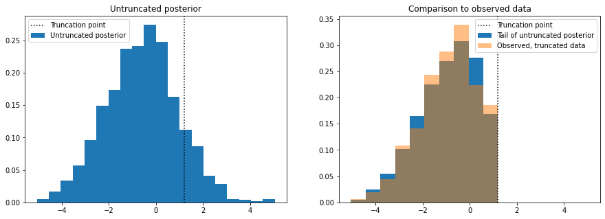
The plot on the left shows data simulated from the posterior distribution with the truncation removed, so we are able to see how the data would look like if it were not truncated. To sense check this, we discard the simulated samples that are above the truncation point and make histogram of those and compare it to a histogram of the true data (right plot).
The TruncatedDistribution class
The source code for the TruncatedNormal in NumPyro uses a class called TruncatedDistribution which abstracts away the logic for sample and log_prob that we will discuss in the next sections. At the moment, though, this logic only works continuous, symmetric distributions with real support.
We can use this class to quickly construct other truncated distributions. For example, if we need a truncated SoftLaplace we can use the following pattern:
[11]:
def TruncatedSoftLaplace(
    loc=0.0, scale=1.0, *, low=None, high=None, validate_args=None
):
    return TruncatedDistribution(
        base_dist=SoftLaplace(loc, scale),
        low=low,
        high=high,
        validate_args=validate_args,
    )
[12]:
def truncated_soft_laplace_model(num_observations, high, x=None):
    loc = numpyro.sample("loc", dist.Normal())
    scale = numpyro.sample("scale", dist.LogNormal())
    with numpyro.plate("obs", num_observations):
        numpyro.sample("x", TruncatedSoftLaplace(loc, scale, high=high), obs=x)
And, as before, we check that we can use this model in the steps of a typical workflow:
[13]:
high = 2.3
num_observations = 200
num_prior_samples = 100

prior = Predictive(truncated_soft_laplace_model, num_samples=num_prior_samples)
prior_samples = prior(PRIOR_RNG, num_observations, high)

true_idx = 0
true_x = prior_samples["x"][true_idx]
true_loc = prior_samples["loc"][true_idx]
true_scale = prior_samples["scale"][true_idx]

mcmc = MCMC(
    NUTS(truncated_soft_laplace_model),
    **MCMC_KWARGS,
)

mcmc.run(
    MCMC_RNG,
    num_observations,
    high,
    true_x,
)

mcmc.print_summary()

print(f"True loc  : {true_loc:3.2}")
print(f"True scale: {true_scale:3.2}")
sample: 100%|█████████████████████████████████████████████████████████████████████████████████████████████████████████████████████████| 4000/4000 [00:02<00:00, 1745.70it/s, 1 steps of size 6.78e-01. acc. prob=0.93]
sample: 100%|█████████████████████████████████████████████████████████████████████████████████████████████████████████████████████████| 4000/4000 [00:00<00:00, 9294.56it/s, 1 steps of size 7.02e-01. acc. prob=0.93]
sample: 100%|████████████████████████████████████████████████████████████████████████████████████████████████████████████████████████| 4000/4000 [00:00<00:00, 10412.30it/s, 1 steps of size 7.20e-01. acc. prob=0.92]
sample: 100%|████████████████████████████████████████████████████████████████████████████████████████████████████████████████████████| 4000/4000 [00:00<00:00, 10583.85it/s, 3 steps of size 7.01e-01. acc. prob=0.93]
                mean       std    median      5.0%     95.0%     n_eff     r_hat
       loc     -0.37      0.17     -0.38     -0.65     -0.10   4034.96      1.00
     scale      1.46      0.12      1.45      1.27      1.65   3618.77      1.00

Number of divergences: 0
True loc  : -0.56
True scale: 1.4
Important
The sample method of the TruncatedDistribution class relies on inverse-transform sampling. This has the implicit requirement that the base distribution should have an icdf method already available. If this is not the case, we will not be able to call the sample method on any instances of our distribution, nor use it with the Predictive class. However, the log_prob method only depends on the cdf
method (which is more frequently available than the icdf). If the log_prob method is available, then we can use our distribution as prior/likelihood in a model.
The FoldedDistribution class
Similar to truncated distributions, NumPyro has the FoldedDistribution class to help you quickly construct folded distributions. Popular examples of folded distributions are the so-called “half-normal”, “half-student” or “half-cauchy”. As the name suggests, these distributions keep only (the positive) half of the distribution. Implicit in the name of these “half” distributions is that they are centered at zero before folding. But, of course, you can fold a distribution even if its not centered at zero. For instance, this is how you would define a folded student-t distribution.
[14]:
def FoldedStudentT(df, loc=0.0, scale=1.0):
    return FoldedDistribution(StudentT(df, loc=loc, scale=scale))
[15]:
def folded_student_model(num_observations, x=None):
    df = numpyro.sample("df", dist.Gamma(6, 2))
    loc = numpyro.sample("loc", dist.Normal())
    scale = numpyro.sample("scale", dist.LogNormal())
    with numpyro.plate("obs", num_observations):
        numpyro.sample("x", FoldedStudentT(df, loc, scale), obs=x)
And we check that we can use our distribution in a typical workflow:
[16]:
# --- prior sampling
num_observations = 500
num_prior_samples = 100
prior = Predictive(folded_student_model, num_samples=num_prior_samples)
prior_samples = prior(PRIOR_RNG, num_observations)


# --- choose any prior sample as the ground truth
true_idx = 0
true_df = prior_samples["df"][true_idx]
true_loc = prior_samples["loc"][true_idx]
true_scale = prior_samples["scale"][true_idx]
true_x = prior_samples["x"][true_idx]

# --- do inference with MCMC
mcmc = MCMC(
    NUTS(folded_student_model),
    **MCMC_KWARGS,
)
mcmc.run(MCMC_RNG, num_observations, true_x)

# --- Check diagostics
mcmc.print_summary()

# --- Compare to ground truth:
print(f"True df   : {true_df:3.2f}")
print(f"True loc  : {true_loc:3.2f}")
print(f"True scale: {true_scale:3.2f}")
sample: 100%|█████████████████████████████████████████████████████████████████████████████████████████████████████████████████████████| 4000/4000 [00:02<00:00, 1343.54it/s, 7 steps of size 3.51e-01. acc. prob=0.75]
sample: 100%|█████████████████████████████████████████████████████████████████████████████████████████████████████████████████████████| 4000/4000 [00:01<00:00, 3644.99it/s, 7 steps of size 3.56e-01. acc. prob=0.73]
sample: 100%|█████████████████████████████████████████████████████████████████████████████████████████████████████████████████████████| 4000/4000 [00:01<00:00, 3137.13it/s, 7 steps of size 2.62e-01. acc. prob=0.91]
sample: 100%|█████████████████████████████████████████████████████████████████████████████████████████████████████████████████████████| 4000/4000 [00:01<00:00, 3028.93it/s, 7 steps of size 1.85e-01. acc. prob=0.96]
                mean       std    median      5.0%     95.0%     n_eff     r_hat
        df      3.12      0.52      3.07      2.30      3.97   2057.60      1.00
       loc     -0.02      0.88     -0.03     -1.28      1.34    925.84      1.01
     scale      2.23      0.21      2.25      1.89      2.57   1677.38      1.00

Number of divergences: 33
True df   : 3.01
True loc  : 0.37
True scale: 2.41
5. Building your own truncated distribution
If the TruncatedDistribution and FoldedDistribution classes are not sufficient to solve your problem, you might want to look into writing your own truncated distribution from the ground up. This can be a tedious process, so this section will give you some guidance and examples to help you with it.
5.1 Recap of NumPyro distributions
A NumPyro distribution should subclass Distribution and implement a few basic ingredients:
Class attributes
The class attributes serve a few different purposes. Here we will mainly care about two:
arg_constraints: Impose some requirements on the parameters of the distribution. Errors are raised at instantiation time if the parameters passed do not satisfy the constraints.support: It is used in some inference algorithms like MCMC and SVI with auto-guides, where we need to perform the algorithm in the unconstrained space. Knowing the support, we can automatically reparametrize things under the hood.
We’ll explain other class attributes as we go.
The __init__ method
This is where we define the parameters of the distribution. We also use jax and lax to promote the parameters to shapes that are valid for broadcasting. The __init__ method of the parent class is also required because that’s where the validation of our parameters is done.
The log_prob method
Implementing the log_prob method ensures that we can do inference. As the name suggests, this method returns the logarithm of the density evaluated at the argument.
The sample method
This method is used for drawing independent samples from our distribution. It is particularly useful for doing prior and posterior predictive checks. Note, in particular, that this method is not needed if you only need to use your distribution as prior in a model - the log_prob method will suffice.
The place-holder code for any of our implementations can be written as
class MyDistribution(Distribution):
    # class attributes
    arg_constraints = {}
    support = None
    def __init__(self):
        pass

    def log_prob(self, value):
        pass

    def sample(self, key, sample_shape=()):
        pass
5.2 Example: Right-truncated normal
We are going to modify a normal distribution so that its new support is of the form (-inf, high), with high a real number. This could be done with the TruncatedNormal distribution but, for the sake of illustration, we are not going to rely on it. We’ll call our distribution RightTruncatedNormal. Let’s write the skeleton code and then proceed to fill in the blanks.
class RightTruncatedNormal(Distribution):
    # <class attributes>
    def __init__(self):
        pass

    def log_prob(self, value):
        pass

    def sample(self, key, sample_shape=()):
        pass
Class attributes
Remember that a non-truncated normal distribution is specified in NumPyro by two parameters, loc and scale, which correspond to the mean and standard deviation. Looking at the source code for the Normal distribution we see the following lines:
arg_constraints = {"loc": constraints.real, "scale": constraints.positive}
support = constraints.real
reparametrized_params = ["loc", "scale"]
The reparametrized_params attribute is used by variational inference algorithms when constructing gradient estimators. The parameters of many common distributions with continuous support (e.g. the Normal distribution) are reparameterizable, while the parameters of discrete distributions are not. Note that reparametrized_params is irrelevant for MCMC algorithms like HMC. See SVI Part III
for more details.
We must adapt these attributes to our case by including the "high" parameter, but there are two issues we need to deal with:
constraints.realis a bit too restrictive. We’d likejnp.infto be a valid value forhigh(equivalent to no truncation), but at the moment infinity is not a valid real number. We deal with this situation by defining our own constraint. The source code forconstraints.realis easy to imitate:
class _RightExtendedReal(constraints.Constraint):
    """
    Any number in the interval (-inf, inf].
    """
    def __call__(self, x):
        return (x == x) & (x != float("-inf"))

    def feasible_like(self, prototype):
        return jnp.zeros_like(prototype)

right_extended_real = _RightExtendedReal()
supportcan no longer be a class attribute as it will depend on the value ofhigh. So instead we implement it as a dependent property.
Our distribution then looks as follows:
class RightTruncatedNormal(Distribution):
    arg_constraints = {
        "loc": constraints.real,
        "scale": constraints.positive,
        "high": right_extended_real,
    }
    reparametrized_params = ["loc", "scale", "high"]

    # ...

    @constraints.dependent_property
    def support(self):
        return constraints.lower_than(self.high)
The __init__ method
Once again we take inspiration from the source code for the normal distribution. The key point is the use of lax and jax to check the shapes of the arguments passed and make sure that such shapes are consistent for broadcasting. We follow the same pattern for our use case – all we need to do is include the high parameter.
In the source implementation of Normal, both parameters loc and scale are given defaults so that one recovers a standard normal distribution if no arguments are specified. In the same spirit, we choose float("inf") as a default for high which would be equivalent to no truncation.
# ...
    def __init__(self, loc=0.0, scale=1.0, high=float("inf"), validate_args=None):
        batch_shape = lax.broadcast_shapes(
            jnp.shape(loc),
            jnp.shape(scale),
            jnp.shape(high),
        )
        self.loc, self.scale, self.high = promote_shapes(loc, scale, high)
        super().__init__(batch_shape, validate_args=validate_args)
# ...
The log_prob method
For a truncated distribution, the log density is given by
where, again, \(p_Z\) is the density of the truncated distribution, \(p_Y\) is the density before truncation, and \(M = \int_T p_Y(y)\mathrm{d}y\). For the specific case of truncating the normal distribution to the interval (-inf, high), the constant \(M\) is equal to the cumulative density evaluated at the truncation point. We can easily implement this log-density method because jax.scipy.stats already has a norm module that we can use.
# ...
    def log_prob(self, value):
        log_m = norm.logcdf(self.high, self.loc, self.scale)
        log_p = norm.logpdf(value, self.loc, self.scale)
        return jnp.where(value < self.high, log_p - log_m, -jnp.inf)
# ...
The sample method
To implement the sample method using inverse-transform sampling, we need to also implement the inverse cumulative distribution function. For this, we can use the ndtri function that lives inside jax.scipy.special. This function returns the inverse cdf for the standard normal distribution. We can do a bit of algebra to obtain the inverse cdf of the truncated, non-standard normal. First recall that if \(X\sim Normal(0, 1)\) and \(Y = \mu + \sigma X\), then
\(Y\sim Normal(\mu, \sigma)\). Then if \(Z\) is the truncated \(Y\), its cumulative density is given by:
And so its inverse is
The translation of the above math into code is
# ...
    def sample(self, key, sample_shape=()):
        shape = sample_shape + self.batch_shape
        minval = jnp.finfo(jnp.result_type(float)).tiny
        u = random.uniform(key, shape, minval=minval)
        return self.icdf(u)


    def icdf(self, u):
        m = norm.cdf(self.high, self.loc, self.scale)
        return self.loc + self.scale * ndtri(m * u)
With everything in place, the final implementation is as below.
[17]:
class _RightExtendedReal(constraints.Constraint):
    """
    Any number in the interval (-inf, inf].
    """

    def __call__(self, x):
        return (x == x) & (x != float("-inf"))

    def feasible_like(self, prototype):
        return jnp.zeros_like(prototype)


right_extended_real = _RightExtendedReal()


class RightTruncatedNormal(Distribution):
    """
    A truncated Normal distribution.
    :param numpy.ndarray loc: location parameter of the untruncated normal
    :param numpy.ndarray scale: scale parameter of the untruncated normal
    :param numpy.ndarray high: point at which the truncation happens
    """

    arg_constraints = {
        "loc": constraints.real,
        "scale": constraints.positive,
        "high": right_extended_real,
    }
    reparametrized_params = ["loc", "scale", "high"]

    def __init__(self, loc=0.0, scale=1.0, high=float("inf"), validate_args=True):
        batch_shape = lax.broadcast_shapes(
            jnp.shape(loc),
            jnp.shape(scale),
            jnp.shape(high),
        )
        self.loc, self.scale, self.high = promote_shapes(loc, scale, high)
        super().__init__(batch_shape, validate_args=validate_args)

    def log_prob(self, value):
        log_m = norm.logcdf(self.high, self.loc, self.scale)
        log_p = norm.logpdf(value, self.loc, self.scale)
        return jnp.where(value < self.high, log_p - log_m, -jnp.inf)

    def sample(self, key, sample_shape=()):
        shape = sample_shape + self.batch_shape
        minval = jnp.finfo(jnp.result_type(float)).tiny
        u = random.uniform(key, shape, minval=minval)
        return self.icdf(u)

    def icdf(self, u):
        m = norm.cdf(self.high, self.loc, self.scale)
        return self.loc + self.scale * ndtri(m * u)

    @constraints.dependent_property
    def support(self):
        return constraints.less_than(self.high)
Let’s try it out!
[18]:
def truncated_normal_model(num_observations, x=None):
    loc = numpyro.sample("loc", dist.Normal())
    scale = numpyro.sample("scale", dist.LogNormal())
    high = numpyro.sample("high", dist.Normal())
    with numpyro.plate("observations", num_observations):
        numpyro.sample("x", RightTruncatedNormal(loc, scale, high), obs=x)
[19]:
num_observations = 1000
num_prior_samples = 100
prior = Predictive(truncated_normal_model, num_samples=num_prior_samples)
prior_samples = prior(PRIOR_RNG, num_observations)
As before, we run mcmc against some synthetic data. We select any random sample from the prior as the ground truth:
[20]:
true_idx = 0
true_loc = prior_samples["loc"][true_idx]
true_scale = prior_samples["scale"][true_idx]
true_high = prior_samples["high"][true_idx]
true_x = prior_samples["x"][true_idx]
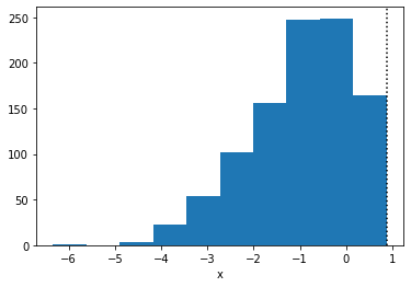
[21]:
plt.hist(true_x.copy())
plt.axvline(true_high, linestyle=":", color="k")
plt.xlabel("x")
plt.show()
Run MCMC and check the estimates:
[22]:
mcmc = MCMC(NUTS(truncated_normal_model), **MCMC_KWARGS)
mcmc.run(MCMC_RNG, num_observations, true_x)
mcmc.print_summary()
sample: 100%|████████████████████████████████████████████████████████████████████████████████████████████████████████████████████████| 4000/4000 [00:02<00:00, 1850.91it/s, 15 steps of size 8.88e-02. acc. prob=0.88]
sample: 100%|█████████████████████████████████████████████████████████████████████████████████████████████████████████████████████████| 4000/4000 [00:00<00:00, 7434.51it/s, 5 steps of size 1.56e-01. acc. prob=0.78]
sample: 100%|████████████████████████████████████████████████████████████████████████████████████████████████████████████████████████| 4000/4000 [00:00<00:00, 7792.94it/s, 54 steps of size 5.41e-02. acc. prob=0.91]
sample: 100%|█████████████████████████████████████████████████████████████████████████████████████████████████████████████████████████| 4000/4000 [00:00<00:00, 7404.07it/s, 9 steps of size 1.77e-01. acc. prob=0.78]
                mean       std    median      5.0%     95.0%     n_eff     r_hat
      high      0.88      0.01      0.88      0.88      0.89    590.13      1.01
       loc     -0.58      0.07     -0.58     -0.70     -0.46    671.04      1.01
     scale      1.40      0.05      1.40      1.32      1.48    678.30      1.01

Number of divergences: 6310
Compare estimates against the ground truth:
[23]:
print(f"True high : {true_high:3.2f}")
print(f"True loc  : {true_loc:3.2f}")
print(f"True scale: {true_scale:3.2f}")
True high : 0.88
True loc  : -0.56
True scale: 1.45
Note that, even though we can recover good estimates for the true values, we had a very high number of divergences. These divergences happen because the data can be outside of the support that we are allowing with our priors. To fix this, we can change the prior on high so that it depends on the observations:
[24]:
def truncated_normal_model_2(num_observations, x=None):
    loc = numpyro.sample("loc", dist.Normal())
    scale = numpyro.sample("scale", dist.LogNormal())
    if x is None:
        high = numpyro.sample("high", dist.Normal())
    else:
        # high is greater or equal to the max value in x:
        delta = numpyro.sample("delta", dist.HalfNormal())
        high = numpyro.deterministic("high", delta + x.max())

    with numpyro.plate("observations", num_observations):
        numpyro.sample("x", RightTruncatedNormal(loc, scale, high), obs=x)
[25]:
mcmc = MCMC(NUTS(truncated_normal_model_2), **MCMC_KWARGS)
mcmc.run(MCMC_RNG, num_observations, true_x)
mcmc.print_summary(exclude_deterministic=False)
sample: 100%|████████████████████████████████████████████████████████████████████████████████████████████████████████████████████████| 4000/4000 [00:03<00:00, 1089.76it/s, 15 steps of size 4.85e-01. acc. prob=0.93]
sample: 100%|█████████████████████████████████████████████████████████████████████████████████████████████████████████████████████████| 4000/4000 [00:00<00:00, 8802.95it/s, 7 steps of size 5.19e-01. acc. prob=0.92]
sample: 100%|█████████████████████████████████████████████████████████████████████████████████████████████████████████████████████████| 4000/4000 [00:00<00:00, 8975.35it/s, 3 steps of size 5.72e-01. acc. prob=0.89]
sample: 100%|████████████████████████████████████████████████████████████████████████████████████████████████████████████████████████| 4000/4000 [00:00<00:00, 8471.94it/s, 15 steps of size 3.76e-01. acc. prob=0.96]
                mean       std    median      5.0%     95.0%     n_eff     r_hat
     delta      0.01      0.01      0.00      0.00      0.01   6104.22      1.00
      high      0.88      0.01      0.88      0.88      0.89   6104.22      1.00
       loc     -0.58      0.08     -0.58     -0.71     -0.46   3319.65      1.00
     scale      1.40      0.06      1.40      1.31      1.49   3377.38      1.00

Number of divergences: 0
And the divergences are gone.
In practice, we usually want to understand how the data would look like without the truncation. To do that in NumPyro, there is no need of writing a separate model, we can simply rely on the condition handler to push the truncation point to infinity:
[26]:
model_without_truncation = numpyro.handlers.condition(
    truncated_normal_model,
    {"high": float("inf")},
)
estimates = mcmc.get_samples().copy()
estimates.pop("high")  # Drop to make sure these are not used
pred = Predictive(
    model_without_truncation,
    posterior_samples=estimates,
)
pred_samples = pred(PRED_RNG, num_observations=1000)
[27]:
# thin the samples for a faster histogram
samples_thinned = pred_samples["x"].ravel()[::1000]
[28]:
f, axes = plt.subplots(1, 2, figsize=(15, 5))

axes[0].hist(
    samples_thinned.copy(), label="Untruncated posterior", bins=20, density=True
)
axes[0].axvline(true_high, linestyle=":", color="k", label="Truncation point")
axes[0].set_title("Untruncated posterior")
axes[0].legend()

axes[1].hist(
    samples_thinned[samples_thinned < true_high].copy(),
    label="Tail of untruncated posterior",
    bins=20,
    density=True,
)
axes[1].hist(true_x.copy(), label="Observed, truncated data", density=True, alpha=0.5)
axes[1].axvline(true_high, linestyle=":", color="k", label="Truncation point")
axes[1].set_title("Comparison to observed data")
axes[1].legend()
plt.show()
5.3 Example: Left-truncated Poisson
As a final example, we now implement a left-truncated Poisson distribution. Note that a right-truncated Poisson could be reformulated as a particular case of a categorical distribution, so we focus on the less trivial case.
Class attributes
For a truncated Poisson we need two parameters, the rate of the original Poisson distribution and a low parameter to indicate the truncation point. As this is a discrete distribution, we need to clarify whether or not the truncation point is included in the support. In this tutorial, we’ll take the convention that the truncation point low is part of the support.
The low parameter has to be given a ‘non-negative integer’ constraint. As it is a discrete parameter, it will not be possible to do inference for this parameter using NUTS. This is likely not a problem since the truncation point is often known in advance. However, if we really must infer the low parameter, it is possible to do so with DiscreteHMCGibbs though one is limited to
using priors with enumerate support.
Like in the case of the truncated normal, the support of this distribution will be defined as a property and not as a class attribute because it depends on the specific value of the low parameter.
class LeftTruncatedPoisson:
    arg_constraints = {
        "low": constraints.nonnegative_integer,
        "rate": constraints.positive,
    }

    # ...
    @constraints.dependent_property(is_discrete=True)
    def support(self):
        return constraints.integer_greater_than(self.low - 1)
The is_discrete argument passed in the dependent_property decorator is used to tell the inference algorithms which variables are discrete latent variables.
The __init__ method
Here we just follow the same pattern as in the previous example.
# ...
def __init__(self, rate=1.0, low=0, validate_args=None):
    batch_shape = lax.broadcast_shapes(
        jnp.shape(low), jnp.shape(rate)
    )
    self.low, self.rate = promote_shapes(low, rate)
    super().__init__(batch_shape, validate_args=validate_args)
# ...
The log_prob method
The logic is very similar to the truncated normal case. But this time we are truncating on the left, so the correct normalization is the complementary cumulative density:
For the code, we can rely on the poisson module that lives inside jax.scipy.stats.
# ...
def log_prob(self, value):
    m = 1 - poisson.cdf(self.low - 1, self.rate)
    log_p = poisson.logpmf(value, self.rate)
    return jnp.where(value >= self.low, log_p - jnp.log(m), -jnp.inf)
# ...
The sample method
Inverse-transform sampling also works for discrete distributions. The “inverse” cdf of a discrete distribution being defined as:
Or, in plain English, \(F^{-1}(u)\) is the highest number for which the cumulative density is less than \(u\). However, there’s currently no implementation of \(F^{-1}\) for the Poisson distribution in Jax (at least, at the moment of writing this tutorial). We have to rely on our own implementation. Fortunately, we can take advantage of the discrete nature of the distribution and easily implement a “brute-force” version that will work for most cases. The brute force approach consists of simply scanning all non-negative integers in order, one by one, until the value of the cumulative density exceeds the argument \(u\). The implicit requirement is that we need a way to evaluate the cumulative density for the truncated distribution, but we can calculate that:
And, of course, the value of \(F_Z(z)\) is equal to zero if \(z < L\). (As in the previous example, we are using \(Y\) to denote the original, un-truncated variable, and we are using \(Z\) to denote the truncated variable)
# ...
def sample(self, key, sample_shape=()):
    shape = sample_shape + self.batch_shape
    minval = jnp.finfo(jnp.result_type(float)).tiny
    u = random.uniform(key, shape, minval=minval)
    return self.icdf(u)

def icdf(self, u):
    def cond_fn(val):
        n, cdf = val
        return jnp.any(cdf < u)

    def body_fn(val):
        n, cdf = val
        n_new = jnp.where(cdf < u, n + 1, n)
        return n_new, self.cdf(n_new)

    low = self.low * jnp.ones_like(u)
    cdf = self.cdf(low)
    n, _ = lax.while_loop(cond_fn, body_fn, (low, cdf))
    return n.astype(jnp.result_type(int))

def cdf(self, value):
    m = 1 - poisson.cdf(self.low - 1, self.rate)
    f = poisson.cdf(value, self.rate) - poisson.cdf(self.low - 1, self.rate)
    return jnp.where(k >= self.low, f / m, 0)
A few comments with respect to the above implementation:
Even with double precision, if
rateis much less thanlow, the above code will not work. Due to numerical limitations, one obtains thatpoisson.cdf(low - 1, rate)is equal (or very close) to1.0. This makes it impossible to re-weight the distribution accurately because the normalization constant would be0.0.The brute-force
icdfis of course very slow, particularly whenrateis high. If you need faster sampling, one option would be to rely on a faster search algorithm. For example:
def icdf_faster(self, u):
    num_bins = 200 # Choose a reasonably large value
    bins = jnp.arange(num_bins)
    cdf = self.cdf(bins)
    indices = jnp.searchsorted(cdf, u)
    return bins[indices]
The obvious limitation here is that the number of bins has to be fixed a priori (jax does not allow for dynamically sized arrays). Another option would be to rely on an approximate implementation, as proposed in this article.
Yet another alternative for the
icdfis to rely onscipy’s implementation and make use of Jax’shost_callbackmodule. This feature allows you to use Python functions without having to code them inJax. This means that we can simply make use ofscipy’s implementation of the Poisson ICDF! From the last equation, we can write the truncated icdf as:
And in python:
def scipy_truncated_poisson_icdf(args): # Note: all arguments are passed inside a tuple
    rate, low, u = args
    rate = np.asarray(rate)
    low = np.asarray(low)
    u = np.asarray(u)
    density = sp_poisson(rate)
    low_cdf = density.cdf(low - 1)
    normalizer = 1.0 - low_cdf
    x = normalizer * u + low_cdf
    return density.ppf(x)
In principle, it wouldn’t be possible to use the above function in our NumPyro distribution because it is not coded in Jax. The jax.experimental.host_callback.call function solves precisely that problem. The code below shows you how to use it, but keep in mind that this is currently an experimental feature so you should expect changes to the module. See the host_callback docs for more details.
# ...
def icdf_scipy(self, u):
    result_shape = jax.ShapeDtypeStruct(
        u.shape,
        jnp.result_type(float) # int type not currently supported
    )
    result = jax.experimental.host_callback.call(
        scipy_truncated_poisson_icdf,
        (self.rate, self.low, u),
        result_shape=result_shape
    )
    return result.astype(jnp.result_type(int))
# ...
Putting it all together, the implementation is as below:
[29]:
def scipy_truncated_poisson_icdf(args):  # Note: all arguments are passed inside a tuple
    rate, low, u = args
    rate = np.asarray(rate)
    low = np.asarray(low)
    u = np.asarray(u)
    density = sp_poisson(rate)
    low_cdf = density.cdf(low - 1)
    normalizer = 1.0 - low_cdf
    x = normalizer * u + low_cdf
    return density.ppf(x)


class LeftTruncatedPoisson(Distribution):
    """
    A truncated Poisson distribution.
    :param numpy.ndarray low: lower bound at which truncation happens
    :param numpy.ndarray rate: rate of the Poisson distribution.
    """

    arg_constraints = {
        "low": constraints.nonnegative_integer,
        "rate": constraints.positive,
    }

    def __init__(self, rate=1.0, low=0, validate_args=None):
        batch_shape = lax.broadcast_shapes(jnp.shape(low), jnp.shape(rate))
        self.low, self.rate = promote_shapes(low, rate)
        super().__init__(batch_shape, validate_args=validate_args)

    def log_prob(self, value):
        m = 1 - poisson.cdf(self.low - 1, self.rate)
        log_p = poisson.logpmf(value, self.rate)
        return jnp.where(value >= self.low, log_p - jnp.log(m), -jnp.inf)

    def sample(self, key, sample_shape=()):
        shape = sample_shape + self.batch_shape
        float_type = jnp.result_type(float)
        minval = jnp.finfo(float_type).tiny
        u = random.uniform(key, shape, minval=minval)
        # return self.icdf(u)        # Brute force
        # return self.icdf_faster(u) # For faster sampling.
        return self.icdf_scipy(u)  # Using `host_callback`

    def icdf(self, u):
        def cond_fn(val):
            n, cdf = val
            return jnp.any(cdf < u)

        def body_fn(val):
            n, cdf = val
            n_new = jnp.where(cdf < u, n + 1, n)
            return n_new, self.cdf(n_new)

        low = self.low * jnp.ones_like(u)
        cdf = self.cdf(low)
        n, _ = lax.while_loop(cond_fn, body_fn, (low, cdf))
        return n.astype(jnp.result_type(int))

    def icdf_faster(self, u):
        num_bins = 200  # Choose a reasonably large value
        bins = jnp.arange(num_bins)
        cdf = self.cdf(bins)
        indices = jnp.searchsorted(cdf, u)
        return bins[indices]

    def icdf_scipy(self, u):
        result_shape = jax.ShapeDtypeStruct(u.shape, jnp.result_type(float))
        result = jax.experimental.host_callback.call(
            scipy_truncated_poisson_icdf,
            (self.rate, self.low, u),
            result_shape=result_shape,
        )
        return result.astype(jnp.result_type(int))

    def cdf(self, value):
        m = 1 - poisson.cdf(self.low - 1, self.rate)
        f = poisson.cdf(value, self.rate) - poisson.cdf(self.low - 1, self.rate)
        return jnp.where(value >= self.low, f / m, 0)

    @constraints.dependent_property(is_discrete=True)
    def support(self):
        return constraints.integer_greater_than(self.low - 1)
Let’s try it out!
[30]:
def discrete_distplot(samples, ax=None, **kwargs):
    """
    Utility function for plotting the samples as a barplot.
    """
    x, y = np.unique(samples, return_counts=True)
    y = y / sum(y)
    if ax is None:
        ax = plt.gca()

    ax.bar(x, y, **kwargs)
    return ax
[31]:
def truncated_poisson_model(num_observations, x=None):
    low = numpyro.sample("low", dist.Categorical(0.2 * jnp.ones((5,))))
    rate = numpyro.sample("rate", dist.LogNormal(1, 1))
    with numpyro.plate("observations", num_observations):
        numpyro.sample("x", LeftTruncatedPoisson(rate, low), obs=x)
Prior samples
[32]:
# -- prior samples
num_observations = 1000
num_prior_samples = 100
prior = Predictive(truncated_poisson_model, num_samples=num_prior_samples)
prior_samples = prior(PRIOR_RNG, num_observations)
Inference
As in the case for the truncated normal, here it is better to replace the prior on the low parameter so that it is consistent with the observed data. We’d like to have a categorical prior on low (so that we can use DiscreteHMCGibbs) whose highest category is equal to the minimum value of x (so that prior and data are consistent). However, we have to be careful in the way we write such model because Jax does not allow for
dynamically sized arrays. A simple way of coding this model is to simply specify the number of categories as an argument:
[33]:
def truncated_poisson_model(num_observations, x=None, k=5):
    zeros = jnp.zeros((k,))
    low = numpyro.sample("low", dist.Categorical(logits=zeros))
    rate = numpyro.sample("rate", dist.LogNormal(1, 1))
    with numpyro.plate("observations", num_observations):
        numpyro.sample("x", LeftTruncatedPoisson(rate, low), obs=x)
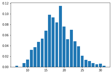
[34]:
# Take any prior sample as the true process.
true_idx = 6
true_low = prior_samples["low"][true_idx]
true_rate = prior_samples["rate"][true_idx]
true_x = prior_samples["x"][true_idx]
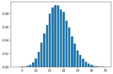
discrete_distplot(true_x.copy());
To do inference, we set k = x.min() + 1. Note also the use of DiscreteHMCGibbs:
[35]:
mcmc = MCMC(DiscreteHMCGibbs(NUTS(truncated_poisson_model)), **MCMC_KWARGS)
mcmc.run(MCMC_RNG, num_observations, true_x, k=true_x.min() + 1)
mcmc.print_summary()
sample: 100%|██████████████████████████████████████████████████████████████████████████████████████████████████████████████████████████| 4000/4000 [00:04<00:00, 808.70it/s, 3 steps of size 9.58e-01. acc. prob=0.93]
sample: 100%|█████████████████████████████████████████████████████████████████████████████████████████████████████████████████████████| 4000/4000 [00:00<00:00, 5916.30it/s, 3 steps of size 9.14e-01. acc. prob=0.93]
sample: 100%|█████████████████████████████████████████████████████████████████████████████████████████████████████████████████████████| 4000/4000 [00:00<00:00, 5082.16it/s, 3 steps of size 9.91e-01. acc. prob=0.92]
sample: 100%|█████████████████████████████████████████████████████████████████████████████████████████████████████████████████████████| 4000/4000 [00:00<00:00, 6511.68it/s, 3 steps of size 8.66e-01. acc. prob=0.94]
                mean       std    median      5.0%     95.0%     n_eff     r_hat
       low      4.13      2.43      4.00      0.00      7.00   7433.79      1.00
      rate     18.16      0.14     18.16     17.96     18.40   3074.46      1.00
[36]:
true_rate
[36]:
DeviceArray(18.2091848, dtype=float64)
As before, one needs to be extra careful when estimating the truncation point. If the truncation point is known is best to provide it.
[37]:
model_with_known_low = numpyro.handlers.condition(
    truncated_poisson_model, {"low": true_low}
)
And note we can use NUTS directly because there’s no need to infer any discrete parameters.
[38]:
mcmc = MCMC(
    NUTS(model_with_known_low),
    **MCMC_KWARGS,
)
[39]:
mcmc.run(MCMC_RNG, num_observations, true_x)
mcmc.print_summary()
sample: 100%|█████████████████████████████████████████████████████████████████████████████████████████████████████████████████████████| 4000/4000 [00:03<00:00, 1185.13it/s, 1 steps of size 9.18e-01. acc. prob=0.93]
sample: 100%|█████████████████████████████████████████████████████████████████████████████████████████████████████████████████████████| 4000/4000 [00:00<00:00, 5786.32it/s, 3 steps of size 1.00e+00. acc. prob=0.92]
sample: 100%|█████████████████████████████████████████████████████████████████████████████████████████████████████████████████████████| 4000/4000 [00:00<00:00, 5919.13it/s, 1 steps of size 8.62e-01. acc. prob=0.94]
sample: 100%|█████████████████████████████████████████████████████████████████████████████████████████████████████████████████████████| 4000/4000 [00:00<00:00, 7562.36it/s, 3 steps of size 9.01e-01. acc. prob=0.93]
                mean       std    median      5.0%     95.0%     n_eff     r_hat
      rate     18.17      0.13     18.17     17.95     18.39   3406.81      1.00

Number of divergences: 0
Removing the truncation
[40]:
model_without_truncation = numpyro.handlers.condition(
    truncated_poisson_model,
    {"low": 0},
)
pred = Predictive(model_without_truncation, posterior_samples=mcmc.get_samples())
pred_samples = pred(PRED_RNG, num_observations)
thinned_samples = pred_samples["x"][::500]
[41]:
discrete_distplot(thinned_samples.copy());