Example: Hilbert space approximation for Gaussian processes.

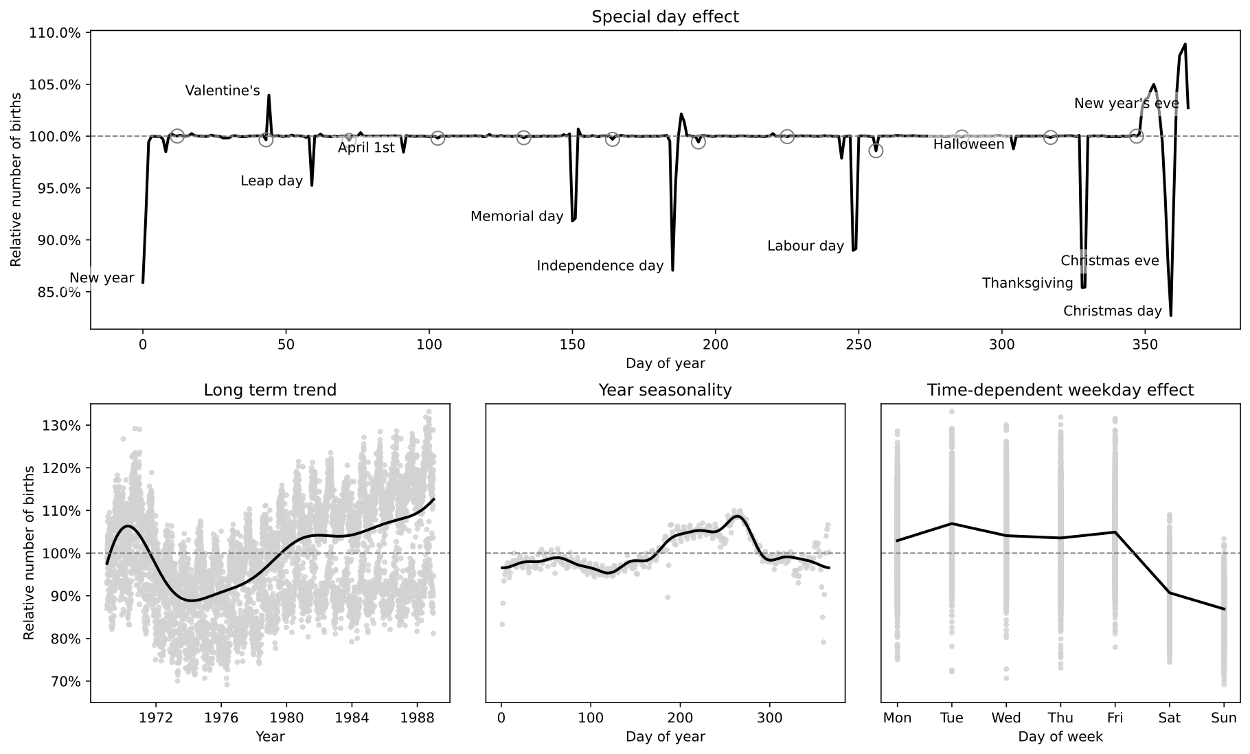
This example replicates the model in the excellent case study by Aki Vehtari [1] (originally written using R and Stan). The case study uses approximate Gaussian processes [2] to model the relative number of births per day in the US from 1969 to 1988. The Hilbert space approximation is way faster than the exact Gaussian processes because it circumvents the need for inverting the covariance matrix.

The original case study also emphasizes the iterative process of building a Bayesian model, which is excellent as a pedagogical resource. Here, however, we replicate only the model that includes all components (long term trend, smooth year seasonality, slowly varying day of week effect, day of the year effect and special floating days effects).

The different components of the model are isolated into separate functions so that they can easily be reused in different contexts. To combine the multiple components into a single birthdays model, here we make use of Numpyro’s scope handler which modifies the site names of the components by adding a prefix to them. By doing this, we avoid duplication of site names within the model. Following this pattern, it is straightforward to construct the other models in [1] with the code provided here.

There are a few minor differences in the mathematical details of our models, which we had to make for the chains to mix properly or for ease of implementation. We have commented on the places where our models are different.

The periodic kernel approximation requires tensorflow-probability on a jax backend. See <https://www.tensorflow.org/probability/examples/TensorFlow_Probability_on_JAX> for installation instructions.

References:

1. Gelman, Vehtari, Simpson, et al (2020), “Bayesian workflow book - Birthdays” <https://avehtari.github.io/casestudies/Birthdays/birthdays.html>.
2. Riutort-Mayol G, Bürkner PC, Andersen MR, et al (2020), “Practical hilbert space approximate bayesian gaussian processes for probabilistic programming”.

import argparse
import os

import matplotlib.pyplot as plt
import pandas as pd

import jax
import jax.numpy as jnp
from tensorflow_probability.substrates import jax as tfp

import numpyro
from numpyro import deterministic, plate, sample
import numpyro.distributions as dist
from numpyro.handlers import scope
from numpyro.infer import MCMC, NUTS, init_to_median


# --- Data processing functions
def get_labour_days(dates):
    """
    First monday of September
    """
    is_september = dates.dt.month.eq(9)
    is_monday = dates.dt.weekday.eq(0)
    is_first_week = dates.dt.day.le(7)

    is_labour_day = is_september & is_monday & is_first_week
    is_day_after = is_labour_day.shift(fill_value=False)

    return is_labour_day | is_day_after


def get_memorial_days(dates):
    """
    Last monday of May
    """
    is_may = dates.dt.month.eq(5)
    is_monday = dates.dt.weekday.eq(0)
    is_last_week = dates.dt.day.ge(25)

    is_memorial_day = is_may & is_monday & is_last_week
    is_day_after = is_memorial_day.shift(fill_value=False)

    return is_memorial_day | is_day_after


def get_thanksgiving_days(dates):
    """
    Third thursday of November
    """
    is_november = dates.dt.month.eq(11)
    is_thursday = dates.dt.weekday.eq(3)
    is_third_week = dates.dt.day.between(22, 28)

    is_thanksgiving = is_november & is_thursday & is_third_week
    is_day_after = is_thanksgiving.shift(fill_value=False)

    return is_thanksgiving | is_day_after


def get_floating_days_indicators(dates):
    def encode(x):
        return jnp.array(x.values, dtype=jnp.result_type(int))

    return {
        "labour_days_indicator": encode(get_labour_days(dates)),
        "memorial_days_indicator": encode(get_memorial_days(dates)),
        "thanksgiving_days_indicator": encode(get_thanksgiving_days(dates)),
    }


def load_data():
    URL = "https://raw.githubusercontent.com/avehtari/casestudies/master/Birthdays/data/births_usa_1969.csv"
    data = pd.read_csv(URL, sep=",")
    day0 = pd.to_datetime("31-Dec-1968")
    dates = [day0 + pd.Timedelta(f"{i}d") for i in data["id"]]
    data["date"] = dates
    data["births_relative"] = data["births"] / data["births"].mean()
    return data


def make_birthdays_data_dict(data):
    x = data["id"].values
    y = data["births_relative"].values
    dates = data["date"]

    xsd = jnp.array((x - x.mean()) / x.std())
    ysd = jnp.array((y - y.mean()) / y.std())
    day_of_week = jnp.array((data["day_of_week"] - 1).values)
    day_of_year = jnp.array((data["day_of_year"] - 1).values)
    floating_days = get_floating_days_indicators(dates)
    period = 365.25
    w0 = x.std() * (jnp.pi * 2 / period)
    L = 1.5 * max(xsd)
    M1 = 10
    M2 = 10  # 20 in original case study
    M3 = 5

    return {
        "x": xsd,
        "day_of_week": day_of_week,
        "day_of_year": day_of_year,
        "w0": w0,
        "L": L,
        "M1": M1,
        "M2": M2,
        "M3": M3,
        **floating_days,
        "y": ysd,
    }


# --- Modelling utility functions --- #
def spectral_density(w, alpha, length):
    c = alpha * jnp.sqrt(2 * jnp.pi) * length
    e = jnp.exp(-0.5 * (length**2) * (w**2))
    return c * e


def diag_spectral_density(alpha, length, L, M):
    sqrt_eigenvalues = jnp.arange(1, 1 + M) * jnp.pi / 2 / L
    return spectral_density(sqrt_eigenvalues, alpha, length)


def eigenfunctions(x, L, M):
    """
    The first `M` eigenfunctions of the laplacian operator in `[-L, L]`
    evaluated at `x`. These are used for the approximation of the
    squared exponential kernel.
    """
    m1 = (jnp.pi / (2 * L)) * jnp.tile(L + x[:, None], M)
    m2 = jnp.diag(jnp.linspace(1, M, num=M))
    num = jnp.sin(m1 @ m2)
    den = jnp.sqrt(L)
    return num / den


def modified_bessel_first_kind(v, z):
    v = jnp.asarray(v, dtype=float)
    return jnp.exp(jnp.abs(z)) * tfp.math.bessel_ive(v, z)


def diag_spectral_density_periodic(alpha, length, M):
    """
    Not actually a spectral density but these are used in the same
    way. These are simply the first `M` coefficients of the low rank
    approximation for the periodic kernel.
    """
    a = length ** (-2)
    J = jnp.arange(0, M)
    c = jnp.where(J > 0, 2, 1)
    q2 = (c * alpha**2 / jnp.exp(a)) * modified_bessel_first_kind(J, a)
    return q2


def eigenfunctions_periodic(x, w0, M):
    """
    Basis functions for the approximation of the periodic kernel.
    """
    m1 = jnp.tile(w0 * x[:, None], M)
    m2 = jnp.diag(jnp.arange(M, dtype=jnp.float32))
    mw0x = m1 @ m2
    cosines = jnp.cos(mw0x)
    sines = jnp.sin(mw0x)
    return cosines, sines


# --- Approximate Gaussian processes --- #
def approx_se_ncp(x, alpha, length, L, M):
    """
    Hilbert space approximation for the squared
    exponential kernel in the non-centered parametrisation.
    """
    phi = eigenfunctions(x, L, M)
    spd = jnp.sqrt(diag_spectral_density(alpha, length, L, M))
    with plate("basis", M):
        beta = sample("beta", dist.Normal(0, 1))

    f = deterministic("f", phi @ (spd * beta))
    return f


def approx_periodic_gp_ncp(x, alpha, length, w0, M):
    """
    Low rank approximation for the periodic squared
    exponential kernel in the non-centered parametrisation.
    """
    q2 = diag_spectral_density_periodic(alpha, length, M)
    cosines, sines = eigenfunctions_periodic(x, w0, M)

    with plate("cos_basis", M):
        beta_cos = sample("beta_cos", dist.Normal(0, 1))

    with plate("sin_basis", M - 1):
        beta_sin = sample("beta_sin", dist.Normal(0, 1))

    # The first eigenfunction for the sine component
    # is zero, so the first parameter wouldn't contribute to the approximation.
    # We set it to zero to identify the model and avoid divergences.
    zero = jnp.array([0.0])
    beta_sin = jnp.concatenate((zero, beta_sin))

    f = deterministic("f", cosines @ (q2 * beta_cos) + sines @ (q2 * beta_sin))
    return f


# --- Components of the Birthdays model --- #
def trend_gp(x, L, M):
    alpha = sample("alpha", dist.HalfNormal(1.0))
    length = sample("length", dist.InverseGamma(10.0, 2.0))
    f = approx_se_ncp(x, alpha, length, L, M)
    return f


def year_gp(x, w0, M):
    alpha = sample("alpha", dist.HalfNormal(1.0))
    length = sample("length", dist.HalfNormal(0.2))  # scale=0.1 in original
    f = approx_periodic_gp_ncp(x, alpha, length, w0, M)
    return f


def weekday_effect(day_of_week):
    with plate("plate_day_of_week", 6):
        weekday = sample("_beta", dist.Normal(0, 1))

    monday = jnp.array([-jnp.sum(weekday)])  # Monday = 0 in original
    beta = deterministic("beta", jnp.concatenate((monday, weekday)))
    return beta[day_of_week]


def yearday_effect(day_of_year):
    slab_df = 50  # 100 in original case study
    slab_scale = 2
    scale_global = 0.1
    tau = sample(
        "tau", dist.HalfNormal(2 * scale_global)
    )  # Original uses half-t with 100df
    c_aux = sample("c_aux", dist.InverseGamma(0.5 * slab_df, 0.5 * slab_df))
    c = slab_scale * jnp.sqrt(c_aux)

    # Jan 1st:  Day 0
    # Feb 29th: Day 59
    # Dec 31st: Day 365
    with plate("plate_day_of_year", 366):
        lam = sample("lam", dist.HalfCauchy(scale=1))
        lam_tilde = jnp.sqrt(c) * lam / jnp.sqrt(c + (tau * lam) ** 2)
        beta = sample("beta", dist.Normal(loc=0, scale=tau * lam_tilde))

    return beta[day_of_year]


def special_effect(indicator):
    beta = sample("beta", dist.Normal(0, 1))
    return beta * indicator


# --- Model --- #
def birthdays_model(
    x,
    day_of_week,
    day_of_year,
    memorial_days_indicator,
    labour_days_indicator,
    thanksgiving_days_indicator,
    w0,
    L,
    M1,
    M2,
    M3,
    y=None,
):
    intercept = sample("intercept", dist.Normal(0, 1))
    f1 = scope(trend_gp, "trend")(x, L, M1)
    f2 = scope(year_gp, "year")(x, w0, M2)
    g3 = scope(trend_gp, "week-trend")(
        x, L, M3
    )  # length ~ lognormal(-1, 1) in original
    weekday = scope(weekday_effect, "week")(day_of_week)
    yearday = scope(yearday_effect, "day")(day_of_year)

    # # --- special days
    memorial = scope(special_effect, "memorial")(memorial_days_indicator)
    labour = scope(special_effect, "labour")(labour_days_indicator)
    thanksgiving = scope(special_effect, "thanksgiving")(thanksgiving_days_indicator)

    day = yearday + memorial + labour + thanksgiving
    # --- Combine components
    f = deterministic("f", intercept + f1 + f2 + jnp.exp(g3) * weekday + day)
    sigma = sample("sigma", dist.HalfNormal(0.5))
    with plate("obs", x.shape[0]):
        sample("y", dist.Normal(f, sigma), obs=y)


# --- plotting function --- #
DATA_STYLE = dict(marker=".", alpha=0.8, lw=0, label="data", c="lightgray")
MODEL_STYLE = dict(lw=2, color="k")


def plot_trend(data, samples, ax=None):
    y = data["births_relative"]
    x = data["date"]
    fsd = samples["intercept"][:, None] + samples["trend/f"]
    f = jnp.quantile(fsd * y.std() + y.mean(), 0.50, axis=0)

    if ax is None:
        ax = plt.gca()

    ax.plot(x, y, **DATA_STYLE)
    ax.plot(x, f, **MODEL_STYLE)
    return ax


def plot_seasonality(data, samples, ax=None):
    y = data["births_relative"]
    sdev = y.std()
    mean = y.mean()
    baseline = (samples["intercept"][:, None] + samples["trend/f"]) * sdev
    y_detrended = y - baseline.mean(0)
    y_year_mean = y_detrended.groupby(data["day_of_year"]).mean()
    x = y_year_mean.index

    f_median = (
        pd.DataFrame(samples["year/f"] * sdev + mean, columns=data["day_of_year"])
        .melt(var_name="day_of_year")
        .groupby("day_of_year")["value"]
        .median()
    )

    if ax is None:
        ax = plt.gca()

    ax.plot(x, y_year_mean, **DATA_STYLE)
    ax.plot(x, f_median, **MODEL_STYLE)
    return ax


def plot_week(data, samples, ax=None):
    if ax is None:
        ax = plt.gca()

    weekdays = ["Mon", "Tue", "Wed", "Thu", "Fri", "Sat", "Sun"]
    y = data["births_relative"]
    x = data["day_of_week"] - 1
    f = jnp.median(samples["week/beta"] * y.std() + y.mean(), 0)

    ax.plot(x, y, **DATA_STYLE)
    ax.plot(range(7), f, **MODEL_STYLE)
    ax.set_xticks(range(7))
    ax.set_xticklabels(weekdays)
    return ax


def plot_weektrend(data, samples, ax=None):
    dates = data["date"]
    weekdays = ["Mon", "Tue", "Wed", "Thu", "Fri", "Sat", "Sun"]
    y = data["births_relative"]
    mean, sdev = y.mean(), y.std()
    intercept = samples["intercept"][:, None]
    f1 = samples["trend/f"]
    f2 = samples["year/f"]
    g3 = samples["week-trend/f"]
    baseline = ((intercept + f1 + f2) * y.std()).mean(0)

    if ax is None:
        ax = plt.gca()

    ax.plot(dates, y - baseline, **DATA_STYLE)
    for n, day in enumerate(weekdays):
        week_beta = samples["week/beta"][:, n][:, None]
        fsd = jnp.exp(g3) * week_beta
        f = jnp.quantile(fsd * sdev + mean, 0.50, axis=0)
        ax.plot(dates, f, **MODEL_STYLE)
        ax.text(dates.iloc[-1], f[-1], day)

    return ax


def plot_1988(data, samples, ax=None):
    indicators = get_floating_days_indicators(data["date"])
    memorial_beta = samples["memorial/beta"][:, None]
    labour_beta = samples["labour/beta"][:, None]
    thanks_beta = samples["thanksgiving/beta"][:, None]

    memorials = indicators["memorial_days_indicator"] * memorial_beta
    labour = indicators["labour_days_indicator"] * labour_beta
    thanksgiving = indicators["thanksgiving_days_indicator"] * thanks_beta
    floating_days = memorials + labour + thanksgiving

    is_1988 = data["date"].dt.year == 1988
    days_in_1988 = data["day_of_year"][is_1988] - 1
    days_effect = samples["day/beta"][:, days_in_1988.values]
    floating_effect = floating_days[:, jnp.argwhere(is_1988.values).ravel()]

    y = data["births_relative"]
    f = (days_effect + floating_effect) * y.std() + y.mean()
    f_median = jnp.median(f, axis=0)

    special_days = {
        "Valentine's": "1988-02-14",
        "Leap day": "1988-02-29",
        "Halloween": "1988-10-31",
        "Christmas eve": "1988-12-24",
        "Christmas day": "1988-12-25",
        "New year": "1988-01-01",
        "New year's eve": "1988-12-31",
        "April 1st": "1988-04-01",
        "Independence day": "1988-07-04",
        "Labour day": "1988-09-05",
        "Memorial day": "1988-05-30",
        "Thanksgiving": "1988-11-24",
    }

    if ax is None:
        ax = plt.gca()

    ax.plot(days_in_1988, f_median, color="k", lw=2)

    for name, date in special_days.items():
        xs = pd.to_datetime(date).day_of_year - 1
        ys = f_median[xs]
        text = ax.text(xs - 3, ys, name, horizontalalignment="right")
        text.set_bbox(dict(facecolor="white", alpha=0.5, edgecolor="none"))

    is_day_13 = data["date"].dt.day == 13
    bad_luck_days = data.loc[is_1988 & is_day_13, "day_of_year"] - 1
    ax.plot(
        bad_luck_days,
        f_median[bad_luck_days.values],
        marker="o",
        mec="gray",
        c="none",
        ms=10,
        lw=0,
    )

    return ax


def make_figure(data, samples):
    import matplotlib.ticker as mtick

    fig = plt.figure(figsize=(15, 9))
    grid = plt.GridSpec(2, 3, wspace=0.1, hspace=0.25)
    axes = (
        plt.subplot(grid[0, :]),
        plt.subplot(grid[1, 0]),
        plt.subplot(grid[1, 1]),
        plt.subplot(grid[1, 2]),
    )
    plot_1988(data, samples, ax=axes[0])
    plot_trend(data, samples, ax=axes[1])
    plot_seasonality(data, samples, ax=axes[2])
    plot_week(data, samples, ax=axes[3])

    for ax in axes:
        ax.axhline(y=1, linestyle="--", color="gray", lw=1)
        if not ax.get_subplotspec().is_first_row():
            ax.set_ylim(0.65, 1.35)

        if not ax.get_subplotspec().is_first_col():
            ax.set_yticks([])
            ax.set_ylabel("")
        else:
            ax.yaxis.set_major_formatter(mtick.PercentFormatter(xmax=1))
            ax.set_ylabel("Relative number of births")

    axes[0].set_title("Special day effect")
    axes[0].set_xlabel("Day of year")
    axes[1].set_title("Long term trend")
    axes[1].set_xlabel("Year")
    axes[2].set_title("Year seasonality")
    axes[2].set_xlabel("Day of year")
    axes[3].set_title("Day of week effect")
    axes[3].set_xlabel("Day of week")
    return fig


# --- functions for running the model --- #
def parse_arguments():
    parser = argparse.ArgumentParser(description="Hilbert space approx for GPs")
    parser.add_argument("--num-samples", nargs="?", default=1000, type=int)
    parser.add_argument("--num-warmup", nargs="?", default=1000, type=int)
    parser.add_argument("--num-chains", nargs="?", default=1, type=int)
    parser.add_argument("--device", default="cpu", type=str, help='use "cpu" or "gpu".')
    parser.add_argument("--x64", action="store_true", help="Enable double precision")
    parser.add_argument(
        "--save-figure",
        default="",
        type=str,
        help="Path where to save the plot with matplotlib.",
    )
    args = parser.parse_args()
    return args


def main(args):
    is_sphinxbuild = "NUMPYRO_SPHINXBUILD" in os.environ
    data = load_data()
    data_dict = make_birthdays_data_dict(data)
    mcmc = MCMC(
        NUTS(birthdays_model, init_strategy=init_to_median),
        num_warmup=args.num_warmup,
        num_samples=args.num_samples,
        num_chains=args.num_chains,
        progress_bar=(not is_sphinxbuild),
    )
    mcmc.run(jax.random.PRNGKey(0), **data_dict)
    if not is_sphinxbuild:
        mcmc.print_summary()

    if args.save_figure:
        samples = mcmc.get_samples()
        print(f"Saving figure at {args.save_figure}")
        fig = make_figure(data, samples)
        fig.savefig(args.save_figure)
        plt.close()

    return mcmc


if __name__ == "__main__":
    args = parse_arguments()
    numpyro.enable_x64(args.x64)
    numpyro.set_platform(args.device)
    numpyro.set_host_device_count(args.num_chains)
    main(args)