Note
Click here to download the full example code
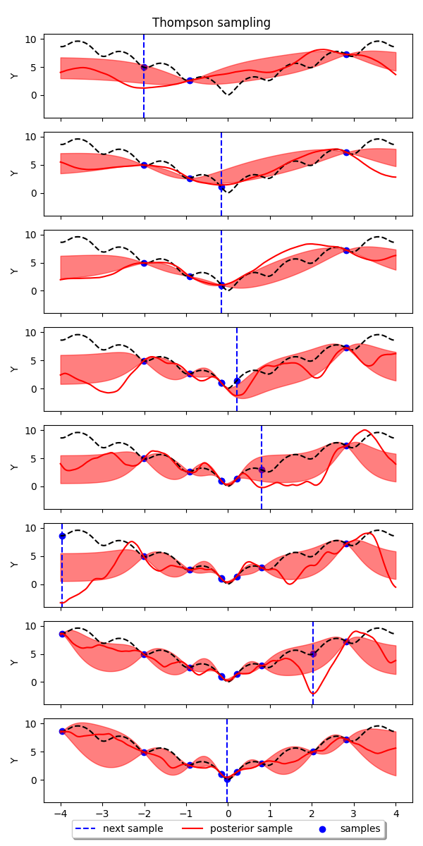
Example: Thompson sampling for Bayesian Optimization with GPs
In this example we show how to implement Thompson sampling for Bayesian optimization with Gaussian processes. The implementation is based on this tutorial: https://gdmarmerola.github.io/ts-for-bayesian-optim/
import argparse

import matplotlib.pyplot as plt
import numpy as np

import jax
import jax.numpy as jnp
import jax.random as random
from jax.scipy import linalg

import numpyro
import numpyro.distributions as dist
from numpyro.infer import SVI, Trace_ELBO
from numpyro.infer.autoguide import AutoDelta

numpyro.enable_x64()


# the function to be minimized. At y=0 to get a 1D cut at the origin
def ackley_1d(x, y=0):
    out = (
        -20 * jnp.exp(-0.2 * jnp.sqrt(0.5 * (x ** 2 + y ** 2)))
        - jnp.exp(0.5 * (jnp.cos(2 * jnp.pi * x) + jnp.cos(2 * jnp.pi * y)))
        + jnp.e
        + 20
    )
    return out


# matern kernel with nu = 5/2
def matern52_kernel(X, Z, var=1.0, length=0.5, jitter=1.0e-6):
    d = jnp.sqrt(0.5) * jnp.sqrt(jnp.power((X[:, None] - Z), 2.0)) / length
    k = var * (1 + d + (d ** 2) / 3) * jnp.exp(-d)
    if jitter:
        # we are assuming a noise free process, but add a small jitter for numerical stability
        k += jitter * jnp.eye(X.shape[0])
    return k


def model(X, Y, kernel=matern52_kernel):
    # set uninformative log-normal priors on our kernel hyperparameters
    var = numpyro.sample("var", dist.LogNormal(0.0, 1.0))
    length = numpyro.sample("length", dist.LogNormal(0.0, 1.0))

    # compute kernel
    k = kernel(X, X, var, length)

    # sample Y according to the standard gaussian process formula
    numpyro.sample(
        "Y",
        dist.MultivariateNormal(loc=jnp.zeros(X.shape[0]), covariance_matrix=k),
        obs=Y,
    )


class GP:
    def __init__(self, kernel=matern52_kernel):
        self.kernel = kernel
        self.kernel_params = None

    def fit(self, X, Y, rng_key, n_step):
        self.X_train = X

        # store moments of training y (to normalize)
        self.y_mean = jnp.mean(Y)
        self.y_std = jnp.std(Y)

        # normalize y
        Y = (Y - self.y_mean) / self.y_std

        # setup optimizer and SVI
        optim = numpyro.optim.Adam(step_size=0.005, b1=0.5)

        svi = SVI(
            model,
            guide=AutoDelta(model),
            optim=optim,
            loss=Trace_ELBO(),
            X=X,
            Y=Y,
        )

        params, _ = svi.run(rng_key, n_step)

        # get kernel parameters from guide with proper names
        self.kernel_params = svi.guide.median(params)

        # store cholesky factor of prior covariance
        self.L = linalg.cho_factor(self.kernel(X, X, **self.kernel_params))

        # store inverted prior covariance multiplied by y
        self.alpha = linalg.cho_solve(self.L, Y)

        return self.kernel_params

    # do GP prediction for a given set of hyperparameters. this makes use of the well-known
    # formula for gaussian process predictions
    def predict(self, X, return_std=False):
        # compute kernels between train and test data, etc.
        k_pp = self.kernel(X, X, **self.kernel_params)
        k_pX = self.kernel(X, self.X_train, **self.kernel_params, jitter=0.0)

        # compute posterior covariance
        K = k_pp - k_pX @ linalg.cho_solve(self.L, k_pX.T)

        # compute posterior mean
        mean = k_pX @ self.alpha

        # we return both the mean function and the standard deviation
        if return_std:
            return (
                (mean * self.y_std) + self.y_mean,
                jnp.sqrt(jnp.diag(K * self.y_std ** 2)),
            )
        else:
            return (mean * self.y_std) + self.y_mean, K * self.y_std ** 2

    def sample_y(self, rng_key, X):
        # get posterior mean and covariance
        y_mean, y_cov = self.predict(X)
        # draw one sample
        return jax.random.multivariate_normal(rng_key, mean=y_mean, cov=y_cov)


# our TS-GP optimizer
class ThompsonSamplingGP:
    """Adapted to numpyro from https://gdmarmerola.github.io/ts-for-bayesian-optim/"""

    # initialization
    def __init__(
        self, gp, n_random_draws, objective, x_bounds, grid_resolution=1000, seed=123
    ):
        # Gaussian Process
        self.gp = gp

        # number of random samples before starting the optimization
        self.n_random_draws = n_random_draws

        # the objective is the function we're trying to optimize
        self.objective = objective

        # the bounds tell us the interval of x we can work
        self.bounds = x_bounds

        # interval resolution is defined as how many points we will use to
        # represent the posterior sample
        # we also define the x grid
        self.grid_resolution = grid_resolution
        self.X_grid = np.linspace(self.bounds[0], self.bounds[1], self.grid_resolution)

        # also initializing our design matrix and target variable
        self.X = np.array([])
        self.y = np.array([])

        self.rng_key = random.PRNGKey(seed)

    # fitting process
    def fit(self, X, y, n_step):
        self.rng_key, subkey = random.split(self.rng_key)
        # fitting the GP
        self.gp.fit(X, y, rng_key=subkey, n_step=n_step)

        # return the fitted model
        return self.gp

    # choose the next Thompson sample
    def choose_next_sample(self, n_step=2_000):

        # if we do not have enough samples, sample randomly from bounds
        if self.X.shape[0] < self.n_random_draws:
            self.rng_key, subkey = random.split(self.rng_key)
            next_sample = random.uniform(
                subkey, minval=self.bounds[0], maxval=self.bounds[1], shape=(1,)
            )

            # define dummy values for sample, mean and std to avoid errors when returning them
            posterior_sample = np.array([np.mean(self.y)] * self.grid_resolution)
            posterior_mean = np.array([np.mean(self.y)] * self.grid_resolution)
            posterior_std = np.array([0] * self.grid_resolution)

        # if we do, we fit the GP and choose the next point based on the posterior draw minimum
        else:

            # 1. Fit the GP to the observations we have
            self.gp = self.fit(self.X, self.y, n_step=n_step)

            # 2. Draw one sample (a function) from the posterior
            self.rng_key, subkey = random.split(self.rng_key)
            posterior_sample = self.gp.sample_y(subkey, self.X_grid)

            # 3. Choose next point as the optimum of the sample
            which_min = np.argmin(posterior_sample)
            next_sample = self.X_grid[which_min]

            # let us also get the std from the posterior, for visualization purposes
            posterior_mean, posterior_std = self.gp.predict(
                self.X_grid, return_std=True
            )

        # let us observe the objective and append this new data to our X and y
        next_observation = self.objective(next_sample)
        self.X = np.append(self.X, next_sample)
        self.y = np.append(self.y, next_observation)

        # returning values of interest
        return (
            self.X,
            self.y,
            self.X_grid,
            posterior_sample,
            posterior_mean,
            posterior_std,
        )


def main(args):
    gp = GP(kernel=matern52_kernel)
    # do inference
    thompson = ThompsonSamplingGP(
        gp, n_random_draws=args.num_random, objective=ackley_1d, x_bounds=(-4, 4)
    )

    fig, axes = plt.subplots(
        args.num_samples - args.num_random, 1, figsize=(6, 12), sharex=True, sharey=True
    )
    for i in range(args.num_samples):
        (
            X,
            y,
            X_grid,
            posterior_sample,
            posterior_mean,
            posterior_std,
        ) = thompson.choose_next_sample(
            n_step=args.num_step,
        )

        if i >= args.num_random:
            ax = axes[i - args.num_random]
            # plot training data
            ax.scatter(X, y, color="blue", marker="o", label="samples")
            ax.axvline(
                X_grid[posterior_sample.argmin()],
                color="blue",
                linestyle="--",
                label="next sample",
            )
            ax.plot(X_grid, ackley_1d(X_grid), color="black", linestyle="--")
            ax.plot(
                X_grid,
                posterior_sample,
                color="red",
                linestyle="-",
                label="posterior sample",
            )
            # plot 90% confidence level of predictions
            ax.fill_between(
                X_grid,
                posterior_mean - posterior_std,
                posterior_mean + posterior_std,
                color="red",
                alpha=0.5,
            )
            ax.set_ylabel("Y")
            if i == args.num_samples - 1:
                ax.set_xlabel("X")

    plt.legend(
        loc="upper center",
        bbox_to_anchor=(0.5, -0.15),
        fancybox=True,
        shadow=True,
        ncol=3,
    )

    fig.suptitle("Thompson sampling")
    fig.tight_layout()
    plt.show()


if __name__ == "__main__":
    assert numpyro.__version__.startswith("0.9.0")
    parser = argparse.ArgumentParser(description="Thompson sampling example")
    parser.add_argument(
        "--num-random", nargs="?", default=2, type=int, help="number of random draws"
    )
    parser.add_argument(
        "--num-samples",
        nargs="?",
        default=10,
        type=int,
        help="number of Thompson samples",
    )
    parser.add_argument(
        "--num-step",
        nargs="?",
        default=2_000,
        type=int,
        help="number of steps for optimization",
    )
    parser.add_argument("--device", default="cpu", type=str, help='use "cpu" or "gpu".')
    args = parser.parse_args()

    numpyro.set_platform(args.device)

    main(args)