Ordinal Regression
Some data are discrete but instrinsically ordered, these are called **ordinal** data. One example is the likert scale for questionairs (“this is an informative tutorial”: 1. strongly disagree / 2. disagree / 3. neither agree nor disagree / 4. agree / 5. strongly agree). Ordinal data is also ubiquitous in the medical world (e.g. the Glasgow Coma Scale for measuring neurological disfunctioning).
This poses a challenge for statistical modeling as the data do not fit the most well known modelling approaches (e.g. linear regression). Modeling the data as categorical is one possibility, but it disregards the inherent ordering in the data, and may be less statistically efficient. There are multiple appoaches for modeling ordered data. Here we will show how to use the OrderedLogistic distribution using cutpoints that are sampled from a Normal distribution with as additional constrain that the cutpoints they are ordered. For a more in-depth discussion of Bayesian modeling of ordinal data, see e.g. Michael Betancour’s blog
[ ]:
!pip install -q numpyro@git+https://github.com/pyro-ppl/numpyro
[1]:
from jax import numpy as np, random
import numpyro
from numpyro import sample
from numpyro.distributions import (Categorical, ImproperUniform, Normal, OrderedLogistic,
                                   TransformedDistribution, constraints, transforms)
from numpyro.infer import MCMC, NUTS
import pandas as pd
import seaborn as sns
assert numpyro.__version__.startswith('0.7.0')
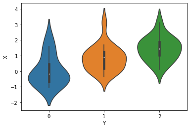
First, generate some data with ordinal structure
[2]:
simkeys  = random.split(random.PRNGKey(1), 2)
nsim     = 50
nclasses = 3
Y        = Categorical(logits=np.zeros(nclasses)).sample(simkeys[0], sample_shape=(nsim,))
X        = Normal().sample(simkeys[1], sample_shape = (nsim,))
X       += Y

print("value counts of Y:")
df = pd.DataFrame({'X': X, 'Y': Y})
print(df.Y.value_counts())

for i in range(nclasses):
    print(f"mean(X) for Y == {i}: {X[np.where(Y==i)].mean():.3f}")
value counts of Y:
1    19
2    16
0    15
Name: Y, dtype: int64
mean(X) for Y == 0: 0.042
mean(X) for Y == 1: 0.832
mean(X) for Y == 2: 1.448
[3]:
sns.violinplot(x='Y', y='X', data=df);
We will model the outcomes Y as coming from an OrderedLogistic distribution, conditional on X. The OrderedLogistic distribution in numpyro requires ordered cutpoints. We can use the ImproperUnifrom distribution to introduce a parameter with an arbitrary support that is otherwise completely uninformative, and then add an ordered_vector constraint.
[4]:
def model1(X, Y, nclasses=3):
    b_X_eta = sample('b_X_eta', Normal(0, 5))
    c_y     = sample('c_y',     ImproperUniform(support=constraints.ordered_vector,
                                                batch_shape=(),
                                                event_shape=(nclasses-1,)))
    with numpyro.plate('obs', X.shape[0]):
        eta = X * b_X_eta
        sample('Y', OrderedLogistic(eta, c_y), obs=Y)

mcmc_key = random.PRNGKey(1234)
kernel = NUTS(model1)
mcmc   = MCMC(kernel, num_warmup=250, num_samples=750)
mcmc.run(mcmc_key, X,Y, nclasses)
mcmc.print_summary()
sample: 100%|██████████| 1000/1000 [00:07<00:00, 126.55it/s, 7 steps of size 4.34e-01. acc. prob=0.95]
                mean       std    median      5.0%     95.0%     n_eff     r_hat
   b_X_eta      1.43      0.35      1.42      0.82      1.96    352.72      1.00
    c_y[0]     -0.11      0.41     -0.11     -0.78      0.55    505.85      1.00
    c_y[1]      2.18      0.52      2.15      1.35      2.95    415.22      1.00

Number of divergences: 0
The ImproperUniform distribution allows us to use parameters with constraints on their domain, without adding any additional information e.g. about the location or scale of the prior distribution on that parameter.
If we want to incorporate such information, for instance that the values of the cut-points should not be too far from zero, we can add an additional sample statement that uses another prior, coupled with an obs argument. In the example below we first sample cutpoints c_y from the ImproperUniform distribution with constraints.ordered_vector as before, and then sample a dummy parameter from a Normal distribution while conditioning on c_y using obs=c_y.
Effectively, we’ve created an improper / unnormalized prior that results from restricting the support of a Normal distribution to the ordered domain
[5]:
def model2(X, Y, nclasses=3):
    b_X_eta = sample('b_X_eta', Normal(0, 5))
    c_y     = sample('c_y',     ImproperUniform(support=constraints.ordered_vector,
                                                batch_shape=(),
                                                event_shape=(nclasses-1,)))
    sample('c_y_smp', Normal(0,1), obs=c_y)
    with numpyro.plate('obs', X.shape[0]):
        eta = X * b_X_eta
        sample('Y', OrderedLogistic(eta, c_y), obs=Y)

kernel = NUTS(model2)
mcmc   = MCMC(kernel, num_warmup=250, num_samples=750)
mcmc.run(mcmc_key, X,Y, nclasses)
mcmc.print_summary()
sample: 100%|██████████| 1000/1000 [00:03<00:00, 315.02it/s, 7 steps of size 4.80e-01. acc. prob=0.94]
                mean       std    median      5.0%     95.0%     n_eff     r_hat
   b_X_eta      1.23      0.30      1.23      0.69      1.65    535.41      1.00
    c_y[0]     -0.25      0.33     -0.25     -0.82      0.27    461.96      1.00
    c_y[1]      1.76      0.38      1.75      1.10      2.33    588.10      1.00

Number of divergences: 0
If having a proper prior for those cutpoints c_y is desirable (e.g. to sample from that prior and get prior predictive), we can use TransformedDistribution with an OrderedTransform transform as follows.
[6]:
def model3(X, Y, nclasses=3):
    b_X_eta = sample('b_X_eta', Normal(0, 5))
    c_y     = sample("c_y",     TransformedDistribution(Normal(0, 1).expand([nclasses - 1]),
                                                        transforms.OrderedTransform()))
    with numpyro.plate('obs', X.shape[0]):
        eta = X * b_X_eta
        sample('Y', OrderedLogistic(eta, c_y), obs=Y)

kernel = NUTS(model3)
mcmc   = MCMC(kernel, num_warmup=250, num_samples=750)
mcmc.run(mcmc_key, X,Y, nclasses)
mcmc.print_summary()
sample: 100%|██████████| 1000/1000 [00:03<00:00, 282.20it/s, 7 steps of size 4.84e-01. acc. prob=0.94]
                mean       std    median      5.0%     95.0%     n_eff     r_hat
   b_X_eta      1.41      0.34      1.40      0.88      2.00    444.42      1.00
    c_y[0]     -0.05      0.36     -0.05     -0.58      0.54    591.60      1.00
    c_y[1]      2.08      0.47      2.07      1.37      2.87    429.27      1.00

Number of divergences: 0