Interactive online version:

Automatic rendering of NumPyro models

In this tutorial we will demonstrate how to create beautiful visualizations of your probabilistic graphical models.

!pip install -q numpyro@git+https://github.com/pyro-ppl/numpyro

from jax import nn
import jax.numpy as jnp

import numpyro
import numpyro.distributions as dist

assert numpyro.__version__.startswith('0.7.2')

A Simple Example

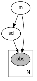
The visualization interface can be readily used with your models:

def model(data):
    m = numpyro.sample('m', dist.Normal(0, 1))
    sd = numpyro.sample('sd', dist.LogNormal(m, 1))
    with numpyro.plate('N', len(data)):
        numpyro.sample('obs', dist.Normal(m, sd), obs=data)

data = jnp.ones(10)
numpyro.render_model(model, model_args=(data,))

The visualization can be saved to a file by providing filename='path' to numpyro.render_model. You can use different formats such as PDF or PNG by changing the filename’s suffix. When not saving to a file (filename=None), you can also change the format with graph.format = 'pdf' where graph is the object returned by numpyro.render_model.

graph = numpyro.render_model(model, model_args=(data,), filename='model.pdf')

Tweaking the visualization

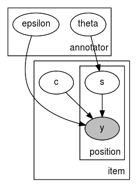
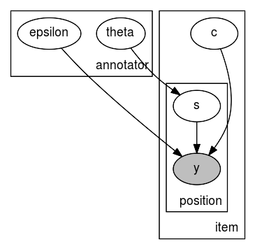
As numpyro.render_model returns an object of type graphviz.dot.Digraph, you can further improve the visualization of this graph. For example, you could use the unflatten preprocessor to improve the layout aspect ratio for more complex models.

def mace(positions, annotations):
    """
    This model corresponds to the plate diagram in Figure 3 of https://www.aclweb.org/anthology/Q18-1040.pdf.
    """
    num_annotators = int(jnp.max(positions)) + 1
    num_classes = int(jnp.max(annotations)) + 1
    num_items, num_positions = annotations.shape

    with numpyro.plate('annotator', num_annotators):
        epsilon = numpyro.sample('epsilon', dist.Dirichlet(jnp.full(num_classes, 10)))
        theta = numpyro.sample('theta', dist.Beta(0.5, 0.5))

    with numpyro.plate('item', num_items, dim=-2):
        # NB: using constant logits for discrete uniform prior
        # (NumPyro does not have DiscreteUniform distribution yet)
        c = numpyro.sample('c', dist.Categorical(logits=jnp.zeros(num_classes)))

        with numpyro.plate('position', num_positions):
            s = numpyro.sample('s', dist.Bernoulli(1 - theta[positions]))
            probs = jnp.where(s[..., None] == 0, nn.one_hot(c, num_classes), epsilon[positions])
            numpyro.sample('y', dist.Categorical(probs), obs=annotations)

positions = jnp.array([1, 1, 1, 2, 3, 4, 5])
annotations = jnp.array([
    [1, 3, 1, 2, 2, 2, 1, 3, 2, 2, 4, 2, 1, 2, 1,
     1, 1, 1, 2, 2, 2, 2, 2, 2, 1, 1, 2, 1, 1, 1,
     1, 3, 1, 2, 2, 4, 2, 2, 3, 1, 1, 1, 2, 1, 2],
    [1, 3, 1, 2, 2, 2, 2, 3, 2, 3, 4, 2, 1, 2, 2,
     1, 1, 1, 2, 2, 2, 2, 2, 2, 1, 1, 3, 1, 1, 1,
     1, 3, 1, 2, 2, 3, 2, 3, 3, 1, 1, 2, 3, 2, 2],
    [1, 3, 2, 2, 2, 2, 2, 3, 2, 2, 4, 2, 1, 2, 1,
     1, 1, 1, 2, 2, 2, 2, 2, 1, 1, 1, 2, 1, 1, 2,
     1, 3, 1, 2, 2, 3, 1, 2, 3, 1, 1, 1, 2, 1, 2],
    [1, 4, 2, 3, 3, 3, 2, 3, 2, 2, 4, 3, 1, 3, 1,
     2, 1, 1, 2, 1, 2, 2, 3, 2, 1, 1, 2, 1, 1, 1,
     1, 3, 1, 2, 3, 4, 2, 3, 3, 1, 1, 2, 2, 1, 2],
    [1, 3, 1, 1, 2, 3, 1, 4, 2, 2, 4, 3, 1, 2, 1,
     1, 1, 1, 2, 3, 2, 2, 2, 2, 1, 1, 2, 1, 1, 1,
     1, 2, 1, 2, 2, 3, 2, 2, 4, 1, 1, 1, 2, 1, 2],
    [1, 3, 2, 2, 2, 2, 1, 3, 2, 2, 4, 4, 1, 1, 1,
     1, 1, 1, 2, 2, 2, 2, 2, 2, 1, 1, 2, 1, 1, 2,
     1, 3, 1, 2, 3, 4, 3, 3, 3, 1, 1, 1, 2, 1, 2],
    [1, 4, 2, 1, 2, 2, 1, 3, 3, 3, 4, 3, 1, 2, 1,
     1, 1, 1, 1, 2, 2, 1, 2, 2, 1, 1, 2, 1, 1, 1,
     1, 3, 1, 2, 2, 3, 2, 3, 2, 1, 1, 1, 2, 1, 2],
]).T

# we subtract 1 because the first index starts with 0 in Python
positions -= 1
annotations -= 1

mace_graph = numpyro.render_model(mace, model_args=(positions, annotations))

# default layout
mace_graph

# layout after processing the layout with unflatten
mace_graph.unflatten(stagger=2)

Distribution annotations

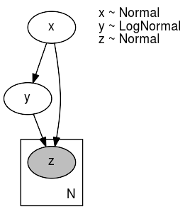
It is possible to display the distribution of each RV in the generated plot by providing render_distributions=True when calling numpyro.render_model.

def model(data):
    x = numpyro.sample('x', dist.Normal(0, 1))
    y = numpyro.sample('y', dist.LogNormal(x, 1))
    with numpyro.plate('N', len(data)):
        numpyro.sample('z', dist.Normal(x, y), obs=data)

data = jnp.ones(10)
numpyro.render_model(model, model_args=(data,), render_distributions=True)