Example: Hilbert space approximation for Gaussian processes.

This example replicates a few of the models in the excellent case study by Aki Vehtari [1] (originally written using R and Stan). The case study uses approximate Gaussian processes [2] to model the relative number of births per day in the US from 1969 to 1988. The Hilbert space approximation is way faster than the exact Gaussian processes because it circumvents the need for inverting the covariance matrix.

The original case study presented by Aki also emphasizes the iterative process of building a Bayesian model, which is excellent as a pedagogical resource. Here, however, we replicate only 4 out of all the models available in [1]. There are a few minor differences in the mathematical details of our models, which we had to make in order for the chains to mix properly. We have clearly commented on the places where our models are different.

References:

1. Gelman, Vehtari, Simpson, et al (2020), “Bayesian workflow book - Birthdays” <https://avehtari.github.io/casestudies/Birthdays/birthdays.html>.
2. Riutort-Mayol G, Bürkner PC, Andersen MR, et al (2020), “Practical hilbert space approximate bayesian gaussian processes for probabilistic programming”.

import argparse
import functools
import operator
import os

import matplotlib.pyplot as plt
import numpy as np
import pandas as pd

import jax
import jax.numpy as jnp
from tensorflow_probability.substrates import jax as tfp

import numpyro
from numpyro import deterministic, plate, sample
import numpyro.distributions as dist
from numpyro.infer import MCMC, NUTS


# --- utility functions
def load_data():
    URL = "https://raw.githubusercontent.com/avehtari/casestudies/master/Birthdays/data/births_usa_1969.csv"
    data = pd.read_csv(URL, sep=",")
    day0 = pd.to_datetime("31-Dec-1968")
    dates = [day0 + pd.Timedelta(f"{i}d") for i in data["id"]]
    data["date"] = dates
    data["births_relative"] = data["births"] / data["births"].mean()
    return data


def save_samples(out_path, samples):
    """
    Save dictionary of arrays using numpys compressed binary format
    Fast reading and writing and efficient storage
    """
    np.savez_compressed(out_path, **samples)


class UnivariateScaler:
    """
    Standardizes the data to have mean 0 and unit standard deviation.
    """

    def __init__(self):
        self._mean = None
        self._std = None

    def fit(self, x):
        self._mean = np.mean(x)
        self._std = np.std(x)
        return self

    def transform(self, x):
        return (x - self._mean) / self._std

    def inverse_transform(self, x):
        return x * self._std + self._mean


def _agg(*args, scaler=None):
    """
    Custom function for aggregating the samples
    and transforming back to the desired scale.
    """
    total = functools.reduce(operator.add, args)
    return (100 * scaler.inverse_transform(total)).mean(axis=0)


# --- modelling functions
def modified_bessel_first_kind(v, z):
    v = jnp.asarray(v, dtype=float)
    return jnp.exp(jnp.abs(z)) * tfp.math.bessel_ive(v, z)


def spectral_density(w, alpha, length):
    c = alpha * jnp.sqrt(2 * jnp.pi) * length
    e = jnp.exp(-0.5 * (length ** 2) * (w ** 2))
    return c * e


def diag_spectral_density(alpha, length, L, M):
    """spd for squared exponential kernel"""
    sqrt_eigenvalues = jnp.arange(1, 1 + M) * jnp.pi / 2 / L
    return spectral_density(sqrt_eigenvalues, alpha, length)


def phi(x, L, M):
    """
    The first `M` eigenfunctions of the laplacian operator in `[-L, L]`
    evaluated at `x`. These are used for the approximation of the
    squared exponential kernel.
    """
    m1 = (jnp.pi / (2 * L)) * jnp.tile(L + x[:, None], M)
    m2 = jnp.diag(jnp.linspace(1, M, num=M))
    num = jnp.sin(m1 @ m2)
    den = jnp.sqrt(L)
    return num / den


def diag_spectral_density_periodic(alpha, length, M):
    """
    Not actually a spectral density but these are used in the same
    way. These are simply the first `M` coefficients of the Taylor
    expansion approximation for the periodic kernel.
    """
    a = length ** (-2)
    J = jnp.arange(1, M + 1)
    q2 = (2 * alpha ** 2 / jnp.exp(a)) * modified_bessel_first_kind(J, a)
    return q2


def phi_periodic(x, w0, M):
    """
    Basis functions for the approximation of the periodic kernel.
    """
    m1 = jnp.tile(w0 * x[:, None], M)
    m2 = jnp.diag(jnp.linspace(1, M, num=M))
    mw0x = m1 @ m2
    return jnp.cos(mw0x), jnp.sin(mw0x)


# --- models
class GP1:
    """
    Long term trend Gaussian process
    """

    def __init__(self):
        self.x_scaler = UnivariateScaler()
        self.y_scaler = UnivariateScaler()

    def model(self, x, L, M, y=None):
        # intercept
        intercept = sample("intercept", dist.Normal(0, 1))

        # long term trend
        ρ = sample("ρ", dist.LogNormal(-1.0, 1.0))
        α = sample("α", dist.HalfNormal(1.0))
        eigenfunctions = phi(x, L, M)
        spd = jnp.sqrt(diag_spectral_density(α, ρ, L, M))

        with plate("basis1", M):
            β1 = sample("β1", dist.Normal(0, 1))

        f1 = deterministic("f1", eigenfunctions @ (spd * β1))
        μ = deterministic("μ", intercept + f1)
        σ = sample("σ", dist.HalfNormal(0.5))
        with plate("n_obs", x.shape[0]):
            sample("y", dist.Normal(μ, σ), obs=y)

    def get_data(self):
        data = load_data()
        x = data["id"].values
        y = data["births_relative"].values
        self.x_scaler.fit(x)
        self.y_scaler.fit(y)
        xsd = jnp.array(self.x_scaler.transform(x))
        ysd = jnp.array(self.y_scaler.transform(y))
        return dict(
            x=xsd,
            y=ysd,
            L=1.5 * max(xsd),
            M=10,
        )

    def make_figure(self, samples):
        data = load_data()
        dates = data["date"]
        y = 100 * data["births_relative"]
        μ = 100 * self.y_scaler.inverse_transform(samples["μ"]).mean(axis=0)

        f = plt.figure(figsize=(15, 5))
        plt.axhline(100, color="k", lw=1, alpha=0.8)
        plt.plot(dates, y, marker=".", lw=0, alpha=0.3)
        plt.plot(dates, μ, color="r", lw=2)
        plt.ylabel("Relative number of births")
        plt.xlabel("")
        return f


class GP2:
    """
    Long term trend with year seasonality component.
    """

    def __init__(self):
        self.x_scaler = UnivariateScaler()
        self.y_scaler = UnivariateScaler()

    def model(self, x, w0, J, L, M, y=None):
        intercept = sample("intercept", dist.Normal(0, 1))

        # long term trend
        ρ1 = sample("ρ1", dist.LogNormal(-1.0, 1.0))
        α1 = sample("α1", dist.HalfNormal(1.0))
        eigenfunctions = phi(x, L, M)
        spd = jnp.sqrt(diag_spectral_density(α1, ρ1, L, M))
        with plate("basis", M):
            β1 = sample("β1", dist.Normal(0, 1))

        # year-periodic component
        ρ2 = sample("ρ2", dist.HalfNormal(0.1))
        α2 = sample("α2", dist.HalfNormal(1.0))
        cosines, sines = phi_periodic(x, w0, J)
        spd_periodic = jnp.sqrt(diag_spectral_density_periodic(α2, ρ2, J))
        with plate("periodic_basis", J):
            β2_cos = sample("β2_cos", dist.Normal(0, 1))
            β2_sin = sample("β2_sin", dist.Normal(0, 1))

        f1 = deterministic("f1", eigenfunctions @ (spd * β1))
        f2 = deterministic(
            "f2", cosines @ (spd_periodic * β2_cos) + sines @ (spd_periodic * β2_sin)
        )
        μ = deterministic("μ", intercept + f1 + f2)
        σ = sample("σ", dist.HalfNormal(0.5))
        with plate("n_obs", x.shape[0]):
            sample("y", dist.Normal(μ, σ), obs=y)

    def get_data(self):
        data = load_data()
        x = data["id"].values
        y = data["births_relative"].values
        self.x_scaler.fit(x)
        self.y_scaler.fit(y)
        xsd = jnp.array(self.x_scaler.transform(x))
        ysd = jnp.array(self.y_scaler.transform(y))
        w0 = 2 * jnp.pi / (365.25 / self.x_scaler._std)
        return dict(
            x=xsd,
            y=ysd,
            w0=w0,
            J=20,
            L=1.5 * max(xsd),
            M=10,
        )

    def make_figure(self, samples):
        data = load_data()
        dates = data["date"]
        y = 100 * data["births_relative"]
        y_by_day_of_year = 100 * data.groupby("day_of_year2")["births_relative"].mean()
        μ = 100 * self.y_scaler.inverse_transform(samples["μ"]).mean(axis=0)
        f1 = 100 * self.y_scaler.inverse_transform(samples["f1"]).mean(axis=0)
        f2 = 100 * self.y_scaler.inverse_transform(samples["f2"]).mean(axis=0)

        fig, axes = plt.subplots(1, 2, figsize=(15, 5))
        axes[0].plot(dates, y, marker=".", lw=0, alpha=0.3)
        axes[0].plot(dates, μ, color="r", lw=2, alpha=1, label="Total")
        axes[0].plot(dates, f1, color="C2", lw=3, alpha=1, label="Trend")

        axes[0].set_ylabel("Relative number of births")
        axes[0].set_title("All time")

        axes[1].plot(
            y_by_day_of_year.index, y_by_day_of_year, marker=".", lw=0, alpha=0.5
        )
        axes[1].plot(
            y_by_day_of_year.index, f2[:366], color="r", lw=2, label="Year seaonality"
        )
        axes[1].set_ylabel("Relative number of births")
        axes[1].set_xlabel("Day of year")
        for ax in axes:
            ax.axhline(100, color="k", lw=1, alpha=0.8)
            ax.legend()

        return fig


class GP3:
    """
    Long term trend with yearly seasonaly and slowly varying day-of-week effect.
    """

    def __init__(self):
        self.x_scaler = UnivariateScaler()
        self.y_scaler = UnivariateScaler()

    def model(self, x, day_of_week, w0, J, L, M, L3, M3, y=None):
        intercept = sample("intercept", dist.Normal(0, 1))

        # long term trend
        ρ1 = sample("ρ1", dist.LogNormal(-1.0, 1.0))
        α1 = sample("α1", dist.HalfNormal(1.0))
        eigenfunctions = phi(x, L, M)
        spd = jnp.sqrt(diag_spectral_density(α1, ρ1, L, M))
        with plate("basis", M):
            β1 = sample("β1", dist.Normal(0, 1))

        # year-periodic component
        ρ2 = sample("ρ2", dist.HalfNormal(0.1))
        α2 = sample("α2", dist.HalfNormal(1.0))
        cosines, sines = phi_periodic(x, w0, J)
        spd_periodic = jnp.sqrt(diag_spectral_density_periodic(α2, ρ2, J))
        with plate("periodic_basis", J):
            β2_cos = sample("β2_cos", dist.Normal(0, 1))
            β2_sin = sample("β2_sin", dist.Normal(0, 1))

        # day of week effect
        with plate("plate_day_of_week", 6):
            β_week = sample("β_week", dist.Normal(0, 1))
        # next enforce sum-to-zero -- this is slightly different from Aki's model,
        # which instead imposes Monday's effect to be zero.
        β_week = jnp.concatenate([jnp.array([-jnp.sum(β_week)]), β_week])

        # long term variation of week effect
        α3 = sample("α3", dist.HalfNormal(0.1))
        ρ3 = sample("ρ3", dist.LogNormal(1.0, 1.0))  # prior: very long-term effect
        eigenfunctions_3 = phi(x, L3, M3)
        spd_3 = jnp.sqrt(diag_spectral_density(α3, ρ3, L3, M3))
        with plate("week_trend", M3):
            β3 = sample("β3", dist.Normal(0, 1))

        # combine
        f1 = deterministic("f1", eigenfunctions @ (spd * β1))
        f2 = deterministic(
            "f2", cosines @ (spd_periodic * β2_cos) + sines @ (spd_periodic * β2_sin)
        )
        g3 = deterministic("g3", eigenfunctions_3 @ (spd_3 * β3))
        μ = deterministic("μ", intercept + f1 + f2 + jnp.exp(g3) * β_week[day_of_week])
        σ = sample("σ", dist.HalfNormal(0.5))
        with plate("n_obs", x.shape[0]):
            sample("y", dist.Normal(μ, σ), obs=y)

    def get_data(self):
        data = load_data()
        x = data["id"].values
        y = data["births_relative"].values
        self.x_scaler.fit(x)
        self.y_scaler.fit(y)
        xsd = jnp.array(self.x_scaler.transform(x))
        ysd = jnp.array(self.y_scaler.transform(y))
        w0 = 2 * jnp.pi / (365.25 / self.x_scaler._std)
        dow = jnp.array(data["day_of_week"].values) - 1
        return dict(
            x=xsd,
            day_of_week=dow,
            w0=w0,
            J=20,
            L=1.5 * max(xsd),
            M=10,
            L3=1.5 * max(xsd),
            M3=5,
            y=ysd,
        )

    def make_figure(self, samples):
        data = load_data()
        dates = data["date"]
        y = 100 * data["births_relative"]
        y_by_day_of_year = 100 * (
            data.groupby("day_of_year2")["births_relative"].mean()
        )
        year_days = y_by_day_of_year.index.values

        μ = samples["μ"]
        intercept = samples["intercept"][:, None]
        f1 = samples["f1"]
        f2 = samples["f2"]
        g3 = samples["g3"]
        β_week = samples["β_week"]
        β_week = np.concatenate([-β_week.sum(axis=1)[:, None], β_week], axis=1)

        fig, axes = plt.subplots(2, 2, figsize=(15, 8), sharey=False, sharex=False)
        axes[0, 0].plot(dates, y, marker=".", lw=0, alpha=0.3)
        axes[0, 0].plot(
            dates,
            _agg(μ, scaler=self.y_scaler),
            color="r",
            lw=0,
            label="Total",
            marker=".",
            alpha=0.5,
        )
        axes[0, 1].plot(dates, y, marker=".", lw=0, alpha=0.3)
        axes[0, 1].plot(
            dates, _agg(f1, scaler=self.y_scaler), color="r", lw=2, label="Trend"
        )
        axes[1, 0].plot(year_days, y_by_day_of_year, marker=".", lw=0, alpha=0.3)
        axes[1, 0].plot(
            year_days,
            _agg(f2[:, :366], scaler=self.y_scaler),
            color="r",
            lw=2,
            label="Year seasonality",
        )
        axes[1, 1].plot(dates, y, marker=".", lw=0, alpha=0.3)
        for day in range(7):
            dow_trend = (jnp.exp(g3).T * β_week[:, day]).T
            fit = _agg(intercept, f1, dow_trend, scaler=self.y_scaler)
            axes[1, 1].plot(dates, fit, lw=2, color="r")

        axes[0, 0].set_title("Total")
        axes[0, 1].set_title("Long term trend")
        axes[1, 0].set_title("Year seasonality")
        axes[1, 1].set_title("Weekly effects with long term trend")
        for ax in axes.flatten():
            ax.axhline(100, color="k", lw=1, alpha=0.8)
            ax.legend()

        return fig


class GP4:
    """
    Long term trend with yearly seasonaly, slowly varying day-of-week effect,
    and special day effect including floating special days.
    """

    def __init__(self):
        self.x_scaler = UnivariateScaler()
        self.y_scaler = UnivariateScaler()

    def model(
        self,
        x,
        day_of_week,
        day_of_year,
        memorial_days_indicator,
        labour_days_indicator,
        thanksgiving_days_indicator,
        w0,
        J,
        L,
        M,
        L3,
        M3,
        y=None,
    ):
        intercept = sample("intercept", dist.Normal(0, 1))

        # long term trend
        ρ1 = sample("ρ1", dist.LogNormal(-1.0, 1.0))
        α1 = sample("α1", dist.HalfNormal(1.0))
        eigenfunctions = phi(x, L, M)
        spd = jnp.sqrt(diag_spectral_density(α1, ρ1, L, M))
        with plate("basis", M):
            β1 = sample("β1", dist.Normal(0, 1))

        # year-periodic component
        ρ2 = sample("ρ2", dist.HalfNormal(0.1))
        α2 = sample("α2", dist.HalfNormal(1.0))
        cosines, sines = phi_periodic(x, w0, J)
        spd_periodic = jnp.sqrt(diag_spectral_density_periodic(α2, ρ2, J))
        with plate("periodic_basis", J):
            β2_cos = sample("β2_cos", dist.Normal(0, 1))
            β2_sin = sample("β2_sin", dist.Normal(0, 1))

        # day of week effect
        with plate("plate_day_of_week", 6):
            β_week = sample("β_week", dist.Normal(0, 1))
        # next enforce sum-to-zero -- this is slightly different from Aki's model,
        # which instead imposes Monday's effect to be zero.
        β_week = jnp.concatenate([jnp.array([-jnp.sum(β_week)]), β_week])

        # long term separation of week effects
        ρ3 = sample("ρ3", dist.LogNormal(1.0, 1.0))
        α3 = sample("α3", dist.HalfNormal(0.1))
        eigenfunctions_3 = phi(x, L3, M3)
        spd_3 = jnp.sqrt(diag_spectral_density(α3, ρ3, L3, M3))
        with plate("week_trend", M3):
            β3 = sample("β3", dist.Normal(0, 1))

        # Finnish horseshoe prior on day of year effect
        # Aki uses slab_df=100 instead, but chains didn't mix
        # in our case for some reason, so we lowered it to 50.
        slab_scale = 2
        slab_df = 50
        scale_global = 0.1
        τ = sample("τ", dist.HalfCauchy(scale=scale_global * 2))
        c_aux = sample("c_aux", dist.InverseGamma(0.5 * slab_df, 0.5 * slab_df))
        c = slab_scale * jnp.sqrt(c_aux)
        with plate("plate_day_of_year", 366):
            λ = sample("λ", dist.HalfCauchy(scale=1))
            λ_tilde = jnp.sqrt(c) * λ / jnp.sqrt(c + (τ * λ) ** 2)
            β4 = sample("β4", dist.Normal(loc=0, scale=τ * λ_tilde))

        # floating special days
        β5_labour = sample("β5_labour", dist.Normal(0, 1))
        β5_memorial = sample("β5_memorial", dist.Normal(0, 1))
        β5_thanksgiving = sample("β5_thanksgiving", dist.Normal(0, 1))

        # combine
        f1 = deterministic("f1", eigenfunctions @ (spd * β1))
        f2 = deterministic(
            "f2", cosines @ (spd_periodic * β2_cos) + sines @ (spd_periodic * β2_sin)
        )
        g3 = deterministic("g3", eigenfunctions_3 @ (spd_3 * β3))
        μ = deterministic(
            "μ",
            intercept
            + f1
            + f2
            + jnp.exp(g3) * β_week[day_of_week]
            + β4[day_of_year]
            + β5_labour * labour_days_indicator
            + β5_memorial * memorial_days_indicator
            + β5_thanksgiving * thanksgiving_days_indicator,
        )
        σ = sample("σ", dist.HalfNormal(0.5))
        with plate("n_obs", x.shape[0]):
            sample("y", dist.Normal(μ, σ), obs=y)

    def _get_floating_days(self, data):
        x = data["id"].values
        memorial_days = data.loc[
            data["date"].dt.month.eq(5)
            & data["date"].dt.weekday.eq(0)
            & data["date"].dt.day.ge(25),
            "id",
        ].values

        labour_days = data.loc[
            data["date"].dt.month.eq(9)
            & data["date"].dt.weekday.eq(0)
            & data["date"].dt.day.le(7),
            "id",
        ].values
        labour_days = np.concatenate((labour_days, labour_days + 1))

        thanksgiving_days = data.loc[
            data["date"].dt.month.eq(11)
            & data["date"].dt.weekday.eq(3)
            & data["date"].dt.day.ge(22)
            & data["date"].dt.day.le(28),
            "id",
        ].values
        thanksgiving_days = np.concatenate((thanksgiving_days, thanksgiving_days + 1))

        md_indicators = np.zeros_like(x)
        md_indicators[memorial_days - 1] = 1
        ld_indicators = np.zeros_like(x)
        ld_indicators[labour_days - 1] = 1
        td_indicators = np.zeros_like(x)
        td_indicators[thanksgiving_days - 1] = 1
        return {
            "memorial_days_indicator": md_indicators,
            "labour_days_indicator": ld_indicators,
            "thanksgiving_days_indicator": td_indicators,
        }

    def get_data(self):
        data = load_data()
        x = data["id"].values
        y = data["births_relative"].values
        self.x_scaler.fit(x)
        self.y_scaler.fit(y)
        xsd = jnp.array(self.x_scaler.transform(x))
        ysd = jnp.array(self.y_scaler.transform(y))
        w0 = 2 * jnp.pi / (365.25 / self.x_scaler._std)
        dow = jnp.array(data["day_of_week"].values) - 1
        doy = jnp.array((data["day_of_year2"] - 1).values)
        return dict(
            x=xsd,
            day_of_week=dow,
            day_of_year=doy,
            w0=w0,
            J=20,
            L=1.5 * max(xsd),
            M=10,
            L3=1.5 * max(xsd),
            M3=5,
            y=ysd,
            **self._get_floating_days(data),
        )

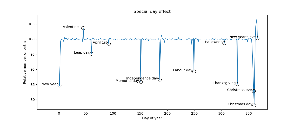
    def make_figure(self, samples):
        special_days = {
            "Valentine's": pd.to_datetime("1988-02-14"),
            "Leap day": pd.to_datetime("1988-02-29"),
            "Halloween": pd.to_datetime("1988-10-31"),
            "Christmas eve": pd.to_datetime("1988-12-24"),
            "Christmas day": pd.to_datetime("1988-12-25"),
            "New year": pd.to_datetime("1988-01-01"),
            "New year's eve": pd.to_datetime("1988-12-31"),
            "April 1st": pd.to_datetime("1988-04-01"),
            "Independence day": pd.to_datetime("1988-07-04"),
            "Labour day": pd.to_datetime("1988-09-05"),
            "Memorial day": pd.to_datetime("1988-05-30"),
            "Thanksgiving": pd.to_datetime("1988-11-24"),
        }
        β4 = samples["β4"]
        β5_labour = samples["β5_labour"]
        β5_memorial = samples["β5_memorial"]
        β5_thanksgiving = samples["β5_thanksgiving"]

        day_effect = np.array(β4)
        md_idx = special_days["Memorial day"].day_of_year - 1
        day_effect[:, md_idx] = day_effect[:, md_idx] + β5_memorial
        ld_idx = special_days["Labour day"].day_of_year - 1
        day_effect[:, ld_idx] = day_effect[:, ld_idx] + β5_labour
        td_idx = special_days["Thanksgiving"].day_of_year - 1
        day_effect[:, td_idx] = day_effect[:, td_idx] + β5_thanksgiving
        day_effect = 100 * day_effect.mean(axis=0)

        fig = plt.figure(figsize=(12, 5))
        plt.plot(np.arange(1, 367), day_effect)
        for name, day in special_days.items():
            xs = day.day_of_year
            ys = day_effect[day.day_of_year - 1]
            plt.plot(xs, ys, marker="o", mec="k", c="none", ms=10)
            plt.text(xs - 3, ys, name, horizontalalignment="right")
        plt.title("Special day effect")
        plt.ylabel("Relative number of births")
        plt.xlabel("Day of year")
        plt.xlim([-40, None])
        return fig


def parse_arguments():
    parser = argparse.ArgumentParser(description="Hilbert space approx for GPs")
    parser.add_argument("--num-samples", nargs="?", default=1000, type=int)
    parser.add_argument("--num-warmup", nargs="?", default=1000, type=int)
    parser.add_argument("--num-chains", nargs="?", default=1, type=int)
    parser.add_argument(
        "--model",
        nargs="?",
        default="tywd",
        help="one of"
        '"t" (Long term trend),'
        '"ty" (t + year seasonality),'
        '"tyw" (t + y + slowly varying weekday effect),'
        '"tywd" (t + y + w + special days effect)',
    )
    parser.add_argument("--device", default="cpu", type=str, help='use "cpu" or "gpu".')
    parser.add_argument("--x64", action="store_true", help="Enable float64 precision")
    parser.add_argument(
        "--save-samples",
        default="",
        type=str,
        help="Path where to store the samples. Must be '.npz' file.",
    )
    parser.add_argument(
        "--save-figure",
        default="",
        type=str,
        help="Path where to save the plot with matplotlib.",
    )
    args = parser.parse_args()
    return args


NAME_TO_MODEL = {
    "t": GP1,
    "ty": GP2,
    "tyw": GP3,
    "tywd": GP4,
}


def main(args):
    is_sphinxbuild = "NUMPYRO_SPHINXBUILD" in os.environ
    model = NAME_TO_MODEL[args.model]()
    data = model.get_data()
    mcmc = MCMC(
        NUTS(model.model),
        num_warmup=args.num_warmup,
        num_samples=args.num_samples,
        num_chains=args.num_chains,
        progress_bar=False if is_sphinxbuild else True,
    )
    mcmc.run(jax.random.PRNGKey(0), **data)
    if not is_sphinxbuild:
        mcmc.print_summary()
    posterior_samples = mcmc.get_samples()
    if args.save_samples:
        print(f"Saving samples at {args.save_samples}")
        save_samples(args.save_samples, posterior_samples)
    if args.save_figure:
        print(f"Saving figure at {args.save_figure}")
        fig = model.make_figure(posterior_samples)
        fig.savefig(args.save_figure)
        plt.close()

    return model, data, mcmc, posterior_samples


if __name__ == "__main__":
    args = parse_arguments()
    if args.x64:
        numpyro.enable_x64()

    numpyro.set_platform(args.device)
    numpyro.set_host_device_count(args.num_chains)
    main(args)